TurbuStat
TurbuStat implements a 14 turbulence-based statistics described in the astronomical literature. TurbuStat also defines a distance metrics for each statistic to quantitatively compare spectral-line data cubes, as well as column density, integrated intensity, or other moment maps.
The source code is hosted here. Contributions to the code base are very much welcome! If you find any issues in the package, please make an issue on github or contact the developers at the email on this page. Thank you!
To be notified of future releases and updates to TurbuStat, please join the mailing list: https://groups.google.com/forum/#!forum/turbustat
If you make use of this package in a publication, please cite our accompanying paper:
@ARTICLE{Koch2019AJ....158....1K,
     author = {{Koch}, Eric W. and {Rosolowsky}, Erik W. and {Boyden}, Ryan D. and
       {Burkhart}, Blakesley and {Ginsburg}, Adam and {Loeppky}, Jason L. and
       {Offner}, Stella S.~R.},
      title = "{TURBUSTAT: Turbulence Statistics in Python}",
    journal = {\aj},
   keywords = {methods: data analysis, methods: statistical, turbulence, Astrophysics - Instrumentation and Methods for Astrophysics},
       year = "2019",
      month = "Jul",
     volume = {158},
     number = {1},
        eid = {1},
      pages = {1},
        doi = {10.3847/1538-3881/ab1cc0},
     eprint = {1904.10484},
     adsurl = {https://ui.adsabs.harvard.edu/abs/2019AJ....158....1K},
    adsnote = {Provided by the SAO/NASA Astrophysics Data System}
    }
If your work makes use of the distance metrics, please cite the following:
@ARTICLE{Koch2017,
 author = {{Koch}, E.~W. and {Ward}, C.~G. and {Offner}, S. and {Loeppky}, J.~L. and {Rosolowsky}, E.~W.},
 title = "{Identifying tools for comparing simulations and observations of spectral-line data cubes}",
 journal = {\mnras},
 archivePrefix = "arXiv",
 eprint = {1707.05415},
 keywords = {methods: statistical, ISM: clouds, radio lines: ISM},
 year = 2017,
 month = oct,
 volume = 471,
 pages = {1506-1530},
 doi = {10.1093/mnras/stx1671},
 adsurl = {http://adsabs.harvard.edu/abs/2017MNRAS.471.1506K},
 adsnote = {Provided by the SAO/NASA Astrophysics Data System}
}
Citations courtesy of ADS
Papers using TurbuStat
TurbuStat Developers
- Eric Koch
- Erik Rosolowsky
- Ryan Boyden
- Blakesley Burkhart
- Adam Ginsburg
- Jason Loeppky
- Stella Offner
- Caleb Ward
Many thanks to everyone who has reported bugs and given feedback on TurbuStat!
- Dario Colombo
- Jesse Feddersen
- Simon Glover
- Jonathan Henshaw
- Sac Medina
- Andrés Izquierdo
Contents:
Installing TurbuStat
The newest release of TurbuStat is available on pip:
>>> pip install turbustat
TurbuStat can also be installed from the github repository.
TurbuStat requires the follow packages:
- astropy>=2.0
- numpy>=1.7
- matplotlib>=1.2
- scipy>=0.12
- sklearn>=0.13.0
- statsmodels>=0.4.0
- scikit-image>=0.12
The following packages are optional when installing TurbuStat and are required only for specific functions in TurbuStat:
- spectral-cube (>v0.4.4) - Efficient handling of PPV cubes. Required for calculating moment arrays in
turbustat.data_reduction.Moments.- radio_beam - A class for handling radio beams and useful utilities. Required for correcting for the beam shape in spatial power spectra. Automatically installed with spectral-cube.
- astrodendro-development - Required for calculating dendrograms in
turbustat.statistics.dendrograms- emcee - MCMC fitting in
PCAand- pyfftw - Wrapper for the FFTW libraries. Allows FFTs to be run in parallel.
- To install TurbuStat, clone the repository::
- Change into the TurbuStat directory and run the following to install TurbuStat::
>>> python setup.py install # doctest: +SKIP
If you find any issues in the installation, please make an issue on github or contact the developers at the email on this page. Thank you!
- To run the testing suite::
>>> MPLBACKEND='agg' python setup.py test # doctest: +SKIP
The matplotlib backend needs to be set to avoid having interactive plots pop up during the tests.
Accepted Data Types
The TurbuStat routines can accept several different data types.
FITS HDU
The most common format is a FITS HDU. These can be loaded in python with the fits library:
>>> from astropy.io import fits
>>> hdulist = fits.open("test.fits")
>>> hdu = hdulist[0]
The TurbuStat statistics expect a single extension for a FITS file to be given.
Numpy array and header
The data can be given as a numpy array, along with a FITS header. This may be useful for data generated from simple physical models (see preparing simulated data). The data can be given as a 2-element tuple or list:
>>> input_data = (array, header)
>>> input_data = [array, header]
Spectral-Cube objects
The spectral-cube package is a dependency of TurbuStat for calculating moment arrays and spectrally regridding cubes for the VCA statistic. When the data need to be preprocessed, it will often be easiest to work with a SpectralCube object. See the spectral-cube tutorial for more information:
>>> from spectral_cube import SpectralCube
>>> cube = SpectralCube("test.fits")
This SpectralCube object can be sliced or used to create moment maps. These spatial 2D maps are called a “Projection” or “Slice” and both are accepted by the TurbuStat statistics:
>>> sliced_img = cube[100]
>>> moment_img = cube.moment0()
The Projection object also offers a number of convenient functions available for a SpectralCube, making it easy to manipulate and alter the data as needed. To load a spatial FITS image as a projection:
>>> from spectral_cube import Projection
>>> img_hdu = fits.open("test_spatial.fits")[0]
>>> proj = Projection.from_hdu(img_hdu)
Preparing Simulated Data
TurbuStat requires the input data be in a valid FITS format. Since simulated observations do not always include a valid observational FITS header, we provide a few convenience functions to create a valid format.
We start with a numpy array of data from some source. First consider a spectral-line data cube with 2 spatial dimensions and one spectral dimension (also called a PPV cube; position-position-velocity). We will need to specify several quantities, like the angular pixel scale, to create the header:
>>> import numpy as np
>>> import astropy.units as u
>>> from turbustat.io.sim_tools import create_fits_hdu
>>> cube = np.ones((8, 16, 16))
>>> pixel_scale = 0.001 * u.deg
>>> spec_pixel_scale = 1000. * u.m / u.s
>>> beamfwhm = 0.003 * u.deg
>>> imshape = cube.shape
>>> restfreq = 1.4 * u.GHz
>>> bunit = u.K
>>> cube_hdu = create_fits_hdu(cube, pixel_scale, spec_pixel_scale, beamfwhm, imshape, restfreq, bunit)
cube_hdu can now be passed to the TurbuStat statistics, or loaded into a spectral_cube.SpectralCube with SpectralCube.read(cube_hdu) for easy manipulation of the PPV cube.
For a two-dimensional image, the FITS HDU can be made in almost the same way, minus spec_pixel_scale:
>>> img = np.ones((16, 16))
>>> imshape = img.shape
>>> img_hdu = create_fits_hdu(img, pixel_scale, beamfwhm, imshape, restfreq, bunit)
The FITS HDU can be given to TurbuStat statistics, or converted to a spectral_cube.Projection with Projection.from_hdu(img_hdu).
You can also create just the FITS headers with:
>>> from turbustat.io.sim_tools import create_image_header, create_cube_header
>>> img_hdr = create_image_header(pixel_scale, beamfwhm, img.shape, restfreq, bunit)
>>> cube_hdr = create_cube_header(pixel_scale, spec_pixel_scale, beamfwhm, cube.shape, restfreq, bunit)
Units
The units should be an equivalent observational unit, depending on the required data product (PPV cube, zeroth moment, centroid, etc…). While TurbuStat does not explicitly check for the input data units, two things should be kept in mind:
- The data cannot be log-scaled.
- When comparing data sets, both should have the same unit. Most statistics are not based on the absolute scale in the data, but it is best to avoid possible misinterpretation of the results.
Noise and missing data
To create realistic data, noise could be added to img and cube in the above examples. The simplest form of noise is Gaussian and can be added to the data with:
>>> sigma = 0.1
>>> noisy_cube = cube + np.random.normal(0., sigma, size=cube.shape)
In this example, Gaussian noise with standard deviation of 0.1 and mean of 0. is added to the cube.
A common observational practice is to mask noise-only regions of an image or data cube. A simple example is, with knowledge of the standard deviation of the noise, to impose an \(N-\sigma\) cut to the data:
>>> N = 3.
>>> # Create a boolean array, where True is above the noise threshold.
>>> signal_mask = noisy_cube > N * sigma
>>> # Set all places below the noise threshold to NaN in the cube
>>> masked_cube = signal_mask.copy()
>>> masked_cube[~signal_mask] = np.NaN
TurbuStat does not contain routines to create robust signal masks. Examples of creating signal masks can be found in Rosolowsky & Leroy 2006 and Dame 2011.
Excluding the dissipation range
When using synthetic observations from simulations, care should be taken to only fit scales in the inertial range. The power-spectrum tutorial shows an example of limiting the fit to the inertial range. The power-spectrum in the dissipation range in that example steepens significantly and is not representative of the turbulent index. This warning should be heeded for power-spectrum-based methods, like the spatial power-spectrum, MVC, VCA and VCS. Spatial structure functions, like the wavelet transform and the delta-variance should also be examined closely for the inflence of the dissipation range on small scales.
Source Code
turbustat.io.sim_tools Module
Functions
create_cube_header(pixel_scale, …[, v0]) |
Create a basic FITS header for a PPV cube. |
create_fits_hdu(data, *header_args) |
Return a FITS hdu for a numpy array of data. |
create_image_header(pixel_scale, beamfwhm, …) |
Create a basic FITS header for an image. |
Data Requirements
Use of the statistics and distance metrics require the input data to satisfy some criteria.
Spatial Projection
TurbuStat assumes that the spatial dimensions of the data are square on the sky. All physical and angular dimensions will be incorrect, otherwise. Data with non-square pixels should first be reprojected. This can be easily done using spectral-cube:
>>> reproj_cube = cube.reproject(new_header)  # doctest: +SKIP
>>> reproj_proj = proj_2D.reproject(new_header_2D)  # doctest: +SKIP
Considerations for distance metrics
The correct pre-processing of data sets is crucial for attaining a meaningful comparison. Listed here are pre-processing considerations that should be considered when using the distance metrics.
The extent of these effects will differ for different data sets. We recommend testing a subset of the data by placing the data at a common resolution (physical or angular) and grid-size, depending on your application. Smoothing and reprojection operations are straightforward to perform with the spectral-cube package.
Spatial scales – Unlike many of the statistics, the distance metrics do not consider physical spatial units. Specifically, metrics that directly compare values at specific scales (
DeltaVariance_Distance,SCF_Distance) will use the given WCS information for the data sets to find a common angular scale.Different spatial sizes are less of a concern for slope-based comparisons, but discrepancies can arise if the data sets have different noise levels. In these cases, the scales used to fit to the power-spectrum (or the equivalent statistic output) should be chosen carefully to avoid bias from the noise. A similar issue can arise when comparing different simulated data sets if the simulations have different inertial ranges.
Spectral scales – The spectral sampling and range should be considered for all methods that utilize the entire PPV cube (SCF, VCA, VCS, dendrograms, PCA, PDF). The issue with using different-sized spectral pixels affects the noise properties, and in some statistics, the measurement itself.
For the former, the noise level can introduce a bias in the measured quantities. To mitigate this, data can be masked prior to running metrics. Otherwise, minimum cut-off values can be specified for metrics that utilize the actual intensity values of the data, such as dendrograms and the PDF. For statistics that are independent of intensity, like a power-law slope or correlation, the fitting range can be specified for each statistic to minimize bias from noise. This is the same effect described above for spatial scales.
For the second case, the VCA index is expected to change with spectral resolution depending on the underlying properties of the turbulent fields (see the VCA tutorial).
Data units for distance metrics
Most of the distance metrics will not depend on the absolute value of the data sets. The exceptions are when values of a statistic are directly compared. This includes Cramer_Distance, the curve distance in DeltaVariance_Distance, and the bins used in the histograms of StatMoments_Distance and PDF_Distance. While each of these methods applies some normalization scheme to the data, we advise converting both data sets to a common unit to minimize possible discrepancies.
Deriving Cube Moments
The Moments class returns moment arrays as well as their errors for use with 2D statistics in the package. Moments are derived using spectral-cube. Definitions for the moments are also available in the spectral-cube documentation.
Basic Use
Moments are easily returned in the expected form for the statistics with Moments. This class takes a FITS file of a spectral-line cube as input and creates moment arrays (zeroth, first, and line width) with their respective uncertainties.:
>>> from turbustat.moments import Moments
>>> # Load in the cube "test.fits"
>>> mm = Moments("test.fits")
>>> mm.make_moments()
>>> mm.make_moment_errors()
>>> output_dict = mm.to_dict()
output_dict is a dictionary that contains keys for the cube and moments. The moment keys contain a list of the moment and its error map.
The moments can also be saved to FITS files. The to_fits function saves FITS files of each moment. The input to the function is the prefix to use in the filenames:
>>> mm.to_fits("test")
This will produce three FITS files: test_moment0.fits, test_centroid.fits, test_linewidth.fits for the zeroth, first, and square-root of the second moments, respectively. These FITS files will contain two extensions, the first with the moment map and the second with the uncertainty map for that moment.
TurbuStat Tutorials
Tutorials are provided for each of the statistic classes and their associated distance metric classes. The tutorials use the same two data sets, described on the data for tutorials page.
The plotting routines are highlighted in each of the tutorials. For users who require custom plotting routines, we recommend looking at the plotting source code as a starting point.
Data for tutorials
Two data sets are used for the tutorials and can be downloaded here. The data are synthetic \(^{13}{\rm CO}(2\rightarrow)1\) spectral-line data cubes from different ENZO adaptive-mesh-refinement simulations. The simulations setup and input parameters are given in Koch et al. 2017 (see Table 1). One of the data sets is a “Fiducial” and the other is a “Design” simulation; the input parameters for the solenoidal fraction, virial parameter, plasma beta, Mach number, and driving scale all differ between the two simulations.
| Parameter | Fiducial | Design |
|---|---|---|
| Solenoidal Fraction | 1/2 | 1/3 |
| Virial Parameter | 6 | 2 |
| Plasma beta | 1 | 2 |
| Mach number | 8.5 | 5 |
| Driving scale | 2-8 | 2-4 |
The simulations were performed on a \(128^3\) base grid with a fixed random turbulent driving field and the boundaries are continuous (i.e., periodic box). The data cubes were produced from one time step after gravity is turned one (\(\sim0.1\) of the free-fall time). The spectral resolution (i.e., channel width) of the cubes is \(40\) m/s.
Moment maps can also be downloaded from the data cubes with the link above. Each data cube has a zeroth (integrated intensity), first (centroid), and square of the second (line width) moment maps.
These data have a limited inertial range, which is evident in the Spatial Power Spectrum tutorial. Turbulent dissipation causes the power-spectrum to steepen on small scales and it is necessary to limit the range of scales that are fit.
The following image shows the integrated intensity (zeroth moment) maps of the tutorial data:
.. image:: images/design_fiducial_moment0.png
Note how the integrated intensity scale varies between the two data sets.
Applying Apodizing Kernels to Data
Applying Fourier transforms to images with emission at the edges can lead to severe ringing effects from the Gibbs phenomenon. This can be an issue for all spatial power-spectra, including the PowerSpectrum, VCA, and MVC.
A common way to avoid this issue is to apply a window function that smoothly tapers the values at the edges of the image to zero (e.g., Stanimirovic et al. 1999). However, the shape of the window function will also affect some frequencies in the Fourier transform. This page demonstrates these effects for some common window shapes.
TurbuStat has four built-in apodizing functions based on the implementations from photutils:
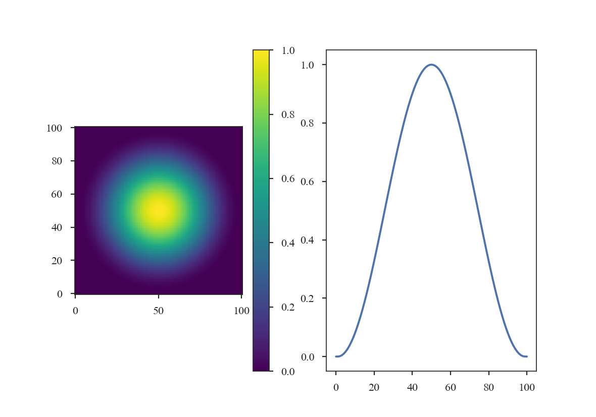
The Hanning window:
>>> from turbustat.statistics.apodizing_kernels import \
...    (CosineBellWindow, TukeyWindow, HanningWindow, SplitCosineBellWindow)
>>> import matplotlib.pyplot as plt
>>> import numpy as np
>>> shape = (101, 101)
>>> taper = HanningWindow()
>>> data = taper(shape)
>>> plt.subplot(121)  # doctest: +SKIP
>>> plt.imshow(data, cmap='viridis', origin='lower')  # doctest: +SKIP
>>> plt.colorbar()  # doctest: +SKIP
>>> plt.subplot(122)  # doctest: +SKIP
>>> plt.plot(data[shape[0] // 2])  # doctest: +SKIP

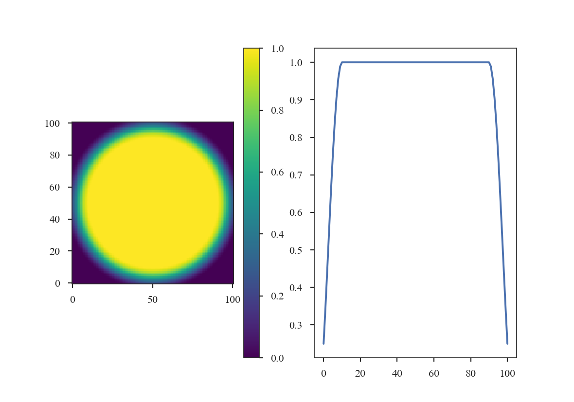
The Cosine Bell Window:
>>> taper2 = CosineBellWindow(alpha=0.8)
>>> data2 = taper2(shape)
>>> plt.subplot(121)  # doctest: +SKIP
>>> plt.imshow(data2, cmap='viridis', origin='lower')  # doctest: +SKIP
>>> plt.colorbar()  # doctest: +SKIP
>>> plt.subplot(122)  # doctest: +SKIP
>>> plt.plot(data2[shape[0] // 2])  # doctest: +SKIP
The Split-Cosine Bell Window:
>>> taper3 = SplitCosineBellWindow(alpha=0.1, beta=0.5)
>>> data3 = taper3(shape)
>>> plt.subplot(121)  # doctest: +SKIP
>>> plt.imshow(data3, cmap='viridis', origin='lower')  # doctest: +SKIP
>>> plt.colorbar()  # doctest: +SKIP
>>> plt.subplot(122)  # doctest: +SKIP
>>> plt.plot(data3[shape[0] // 2])  # doctest: +SKIP
And the Tukey Window:
>>> taper4 = TukeyWindow(alpha=0.3)
>>> data4 = taper4(shape)
>>> plt.subplot(121)  # doctest: +SKIP
>>> plt.imshow(data4, cmap='viridis', origin='lower')  # doctest: +SKIP
>>> plt.colorbar()  # doctest: +SKIP
>>> plt.subplot(122)  # doctest: +SKIP
>>> plt.plot(data4[shape[0] // 2])  # doctest: +SKIP
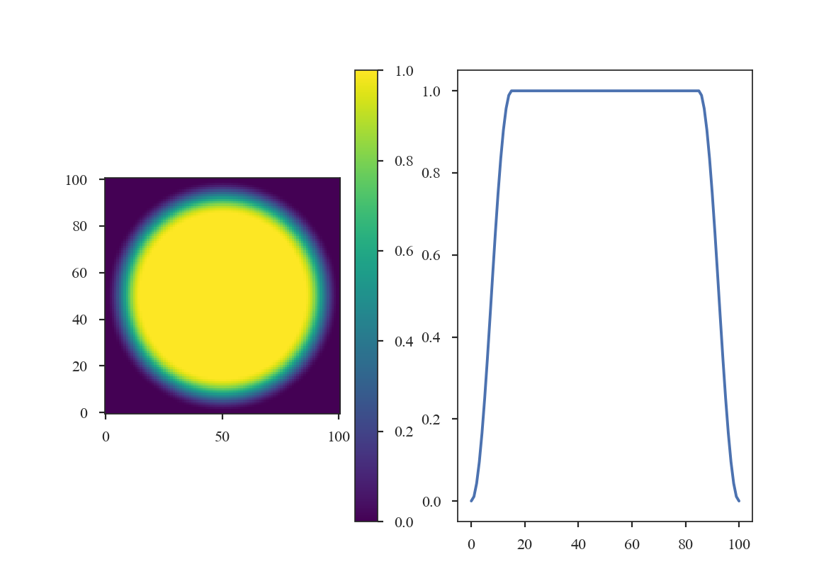
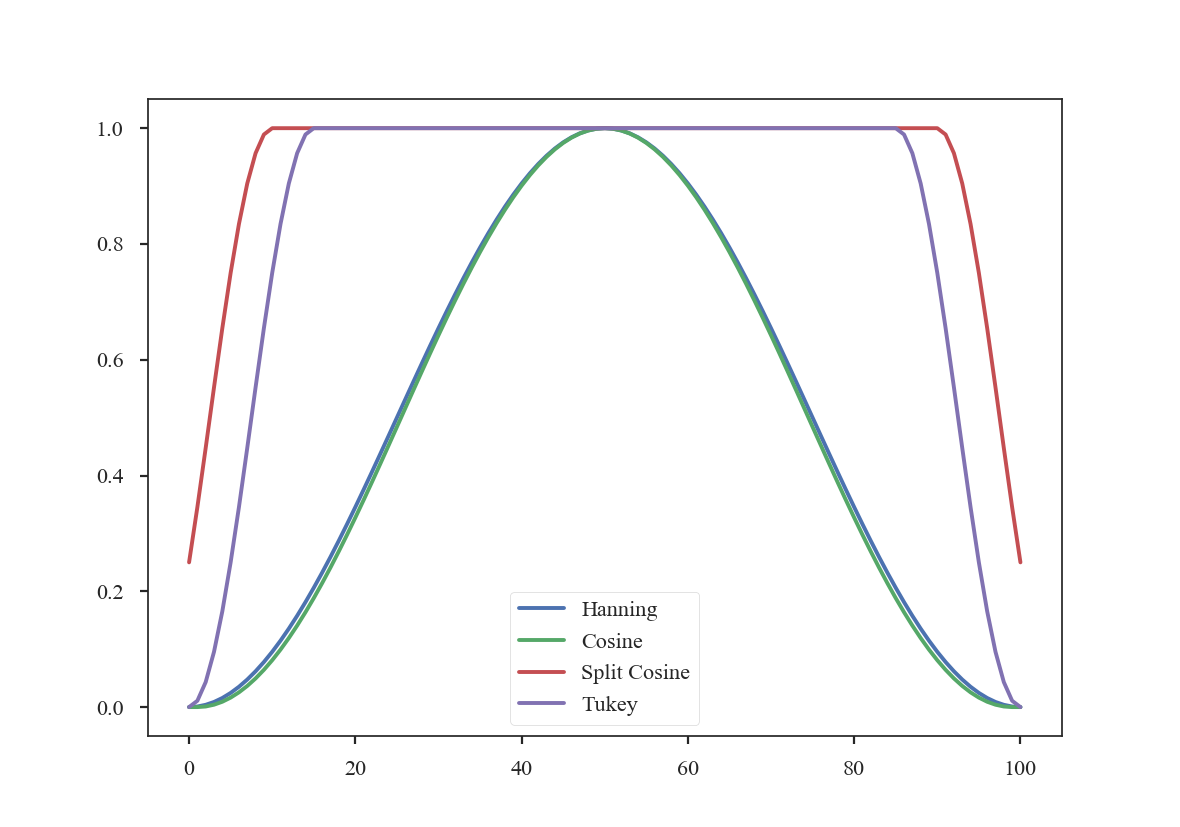
The former two windows consistently taper smoothly from the centre to the edge, while the latter two have flattened plateaus with tapering only at the edge. Plotting the 1-dimensional slices makes these differences clear:
>>> plt.plot(data[shape[0] // 2], label='Hanning')  # doctest: +SKIP
>>> plt.plot(data2[shape[0] // 2], label='Cosine')  # doctest: +SKIP
>>> plt.plot(data3[shape[0] // 2], label='Split Cosine')  # doctest: +SKIP
>>> plt.plot(data4[shape[0] // 2], label='Tukey')  # doctest: +SKIP
>>> plt.legend(frameon=True)  # doctest: +SKIP
To get an idea of how these apodizing functions affect the data, we can examine their power-spectra:
>>> freqs = np.fft.rfftfreq(shape[0])
>>> plt.loglog(freqs, np.abs(np.fft.rfft(data[shape[0] // 2]))**2, label='Hanning')  # doctest: +SKIP
>>> plt.loglog(freqs, np.abs(np.fft.rfft(data2[shape[0] // 2]))**2, label='Cosine')  # doctest: +SKIP
>>> plt.loglog(freqs, np.abs(np.fft.rfft(data3[shape[0] // 2]))**2, label='Split Cosine')  # doctest: +SKIP
>>> plt.loglog(freqs, np.abs(np.fft.rfft(data4[shape[0] // 2]))**2, label='Tukey')  # doctest: +SKIP
>>> plt.legend(frameon=True)  # doctest: +SKIP
>>> plt.xlabel("Freq. (1 / pix)")  # doctest: +SKIP
>>> plt.ylabel("Power")  # doctest: +SKIP
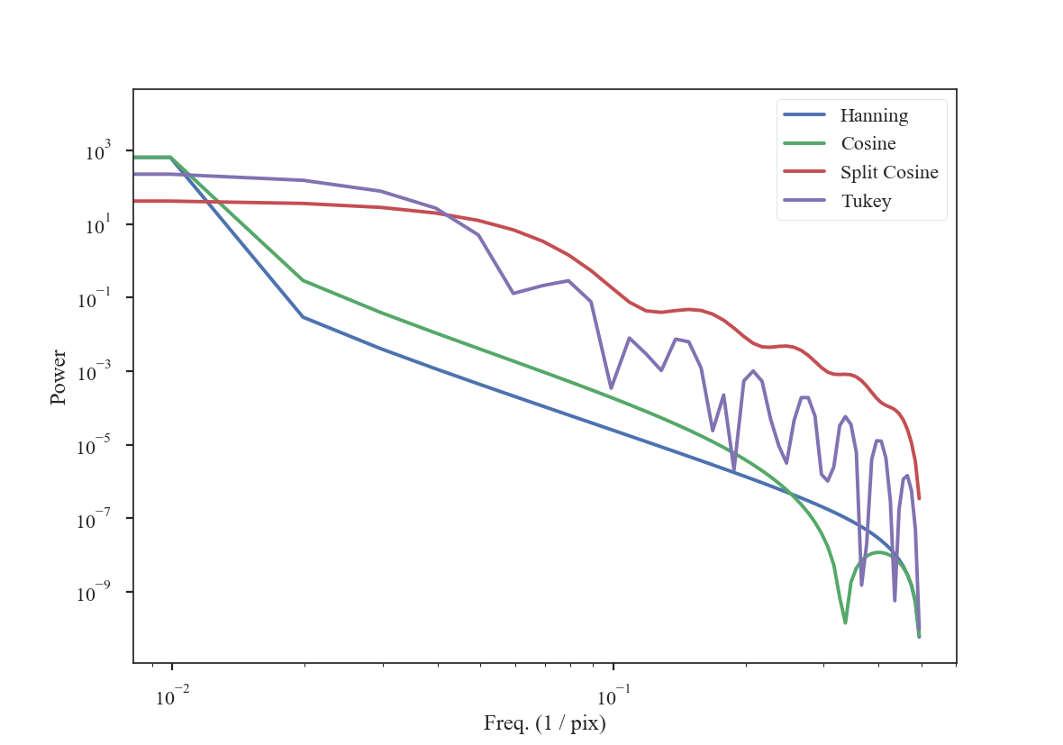
The smoothly-varying windows (Hanning and Cosine) have power-spectra that consistently decrease the power. This means that the use of a Hanning or Cosine window will affect the shape of power-spectra over a larger range of frequencies than the Split-Cosine or Tukey windows.
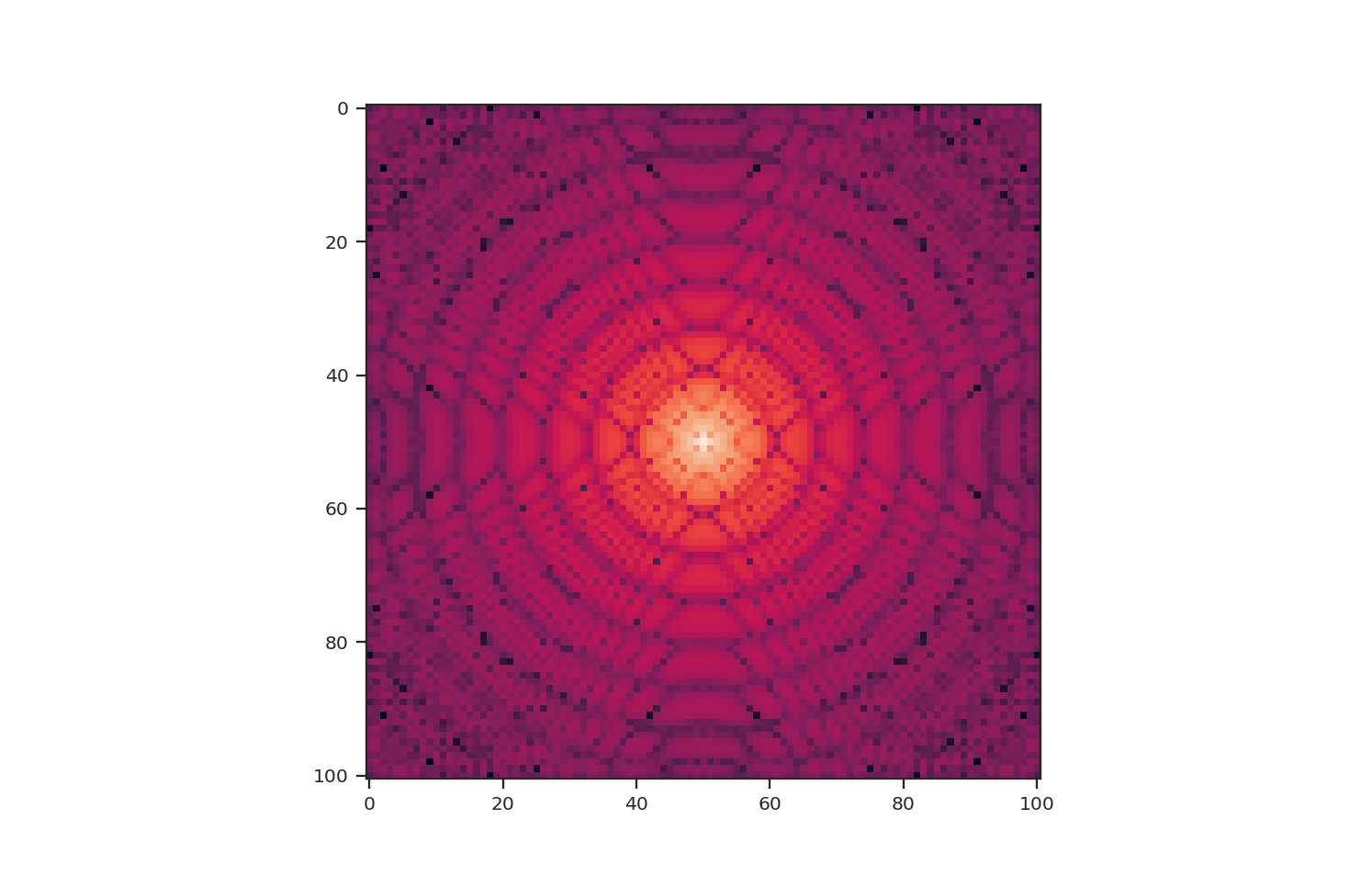
These apodizing kernels are azimuthally-symmetric. However, as an example, the 2D power-spectrum of the Tukey Window, which is used below, has this structure:
>>> plt.imshow(np.log10(np.fft.fftshift(np.abs(np.fft.fft2(data4))**2)))
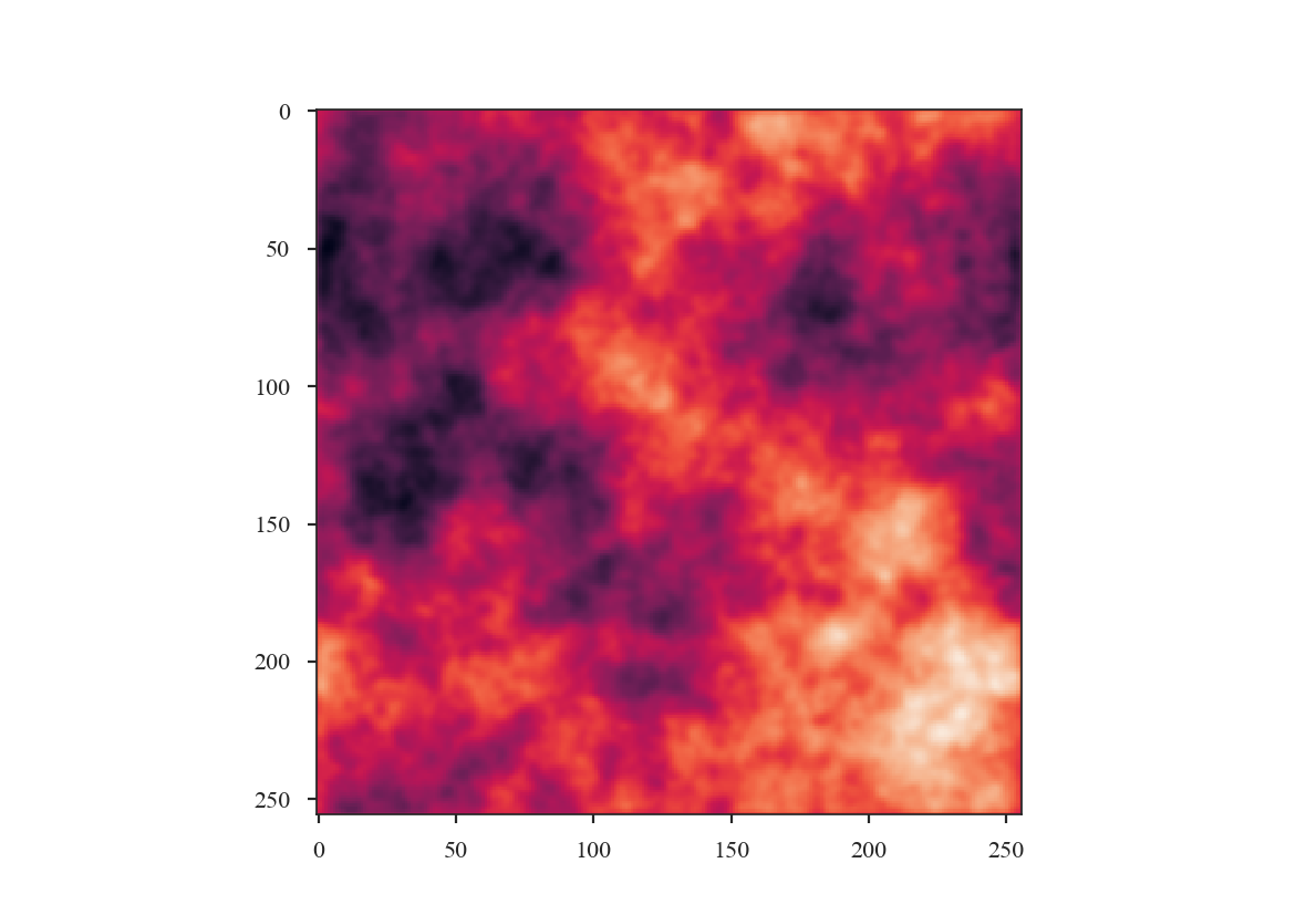
As an example, we will compare the effect each of the windows has on a red-noise image.
>>> from turbustat.simulator import make_extended
>>> from turbustat.io.sim_tools import create_fits_hdu
>>> from astropy import units as u
>>> # Image drawn from red-noise
>>> rnoise_img = make_extended(256, powerlaw=3.)
>>> # Define properties to generate WCS information
>>> pixel_scale = 3 * u.arcsec
>>> beamfwhm = 3 * u.arcsec
>>> imshape = rnoise_img.shape
>>> restfreq = 1.4 * u.GHz
>>> bunit = u.K
>>> # Create a FITS HDU
>>> plaw_hdu = create_fits_hdu(rnoise_img, pixel_scale, beamfwhm, imshape, restfreq, bunit)
>>> plt.imshow(plaw_hdu.data)  # doctest: +SKIP

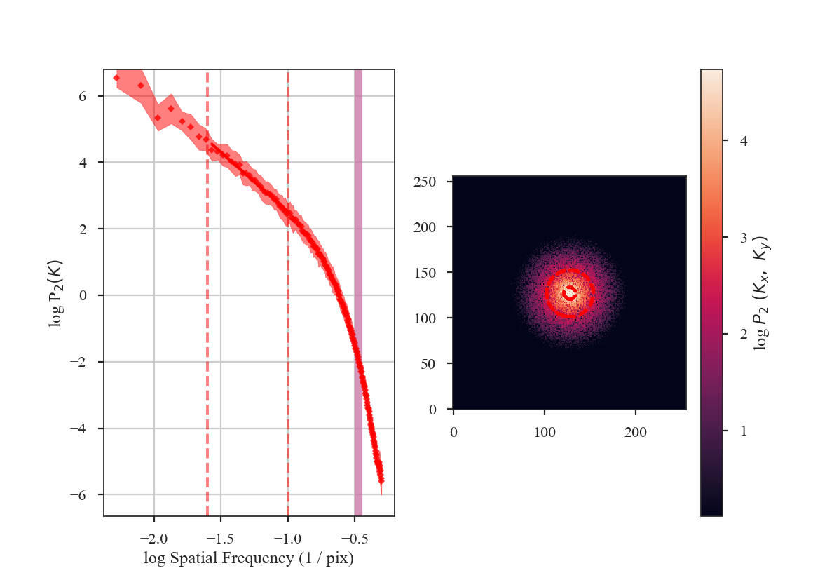
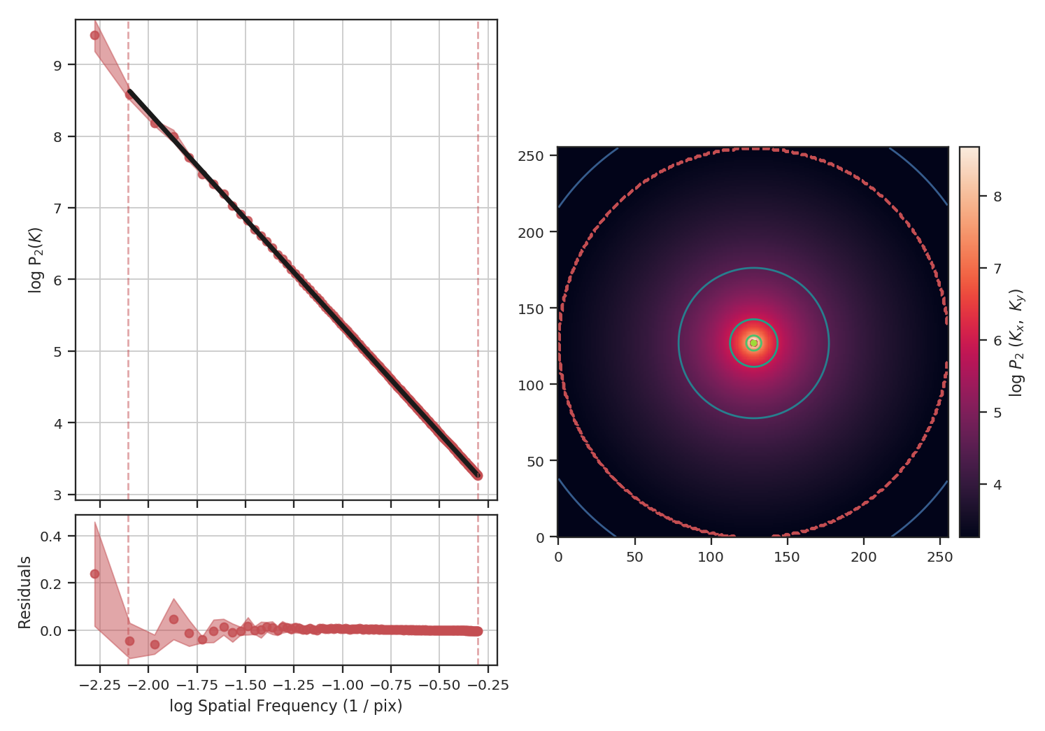
The image should have a power-spectrum index of 3 with mean values centred at 0. By running PowerSpectrum, we can confirm that the index is indeed 3 (see the variable x1 in the output):
>>> from turbustat.statistics import PowerSpectrum
>>> pspec = PowerSpectrum(plaw_hdu)
>>> pspec.run(verbose=True, radial_pspec_kwargs={'binsize': 1.0},
...           fit_2D=False,
...           low_cut=1. / (60 * u.pix))  # doctest: +SKIP
                            OLS Regression Results
==============================================================================
Dep. Variable:                      y   R-squared:                       1.000
Model:                            OLS   Adj. R-squared:                  1.000
Method:                 Least Squares   F-statistic:                 8.070e+06
Date:                Thu, 21 Jun 2018   Prob (F-statistic):               0.00
Time:                        11:43:47   Log-Likelihood:                 701.40
No. Observations:                 177   AIC:                            -1399.
Df Residuals:                     175   BIC:                            -1392.
Df Model:                           1
Covariance Type:            nonrobust
==============================================================================
                 coef    std err          t      P>|t|      [0.025      0.975]
------------------------------------------------------------------------------
const          0.0032      0.001      3.952      0.000       0.002       0.005
x1            -2.9946      0.001  -2840.850      0.000      -2.997      -2.992
==============================================================================
Omnibus:                      252.943   Durbin-Watson:                   1.077
Prob(Omnibus):                  0.000   Jarque-Bera (JB):            26797.433
Skew:                          -5.963   Prob(JB):                         0.00
Kurtosis:                      62.087   Cond. No.                         4.55
==============================================================================
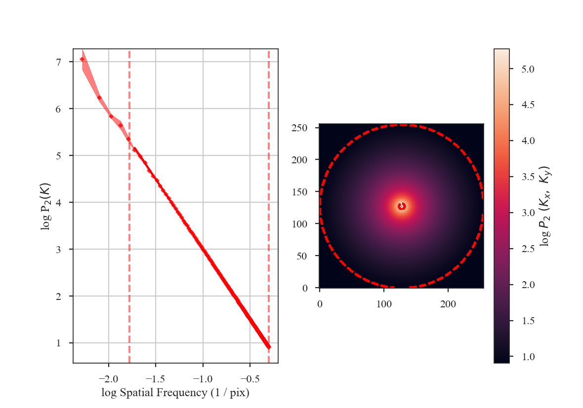
The slope is nearly 3, as expected. Note that we have limited the range of frequencies fit over to avoid the largest scales using the parameter low_cut. Also note that there is a “hole” in the centre of the 2D power-spectrum on the right panel in the image. This is the zero-frequency of the image and scales with the mean value of the image. Since this image is centred at 0, there is no power at the zero-frequency point in the centre of the 2D power-spectrum.
From the figure, it is clear that the samples on larger scales deviate from a power-law. This deviation is a result of the lack of samples on these large-scales. It can be avoided by increasing the size of the radial bins, but we will use small bins here to highlight the effect of the apodizing kernels on the power-spectrum shape.
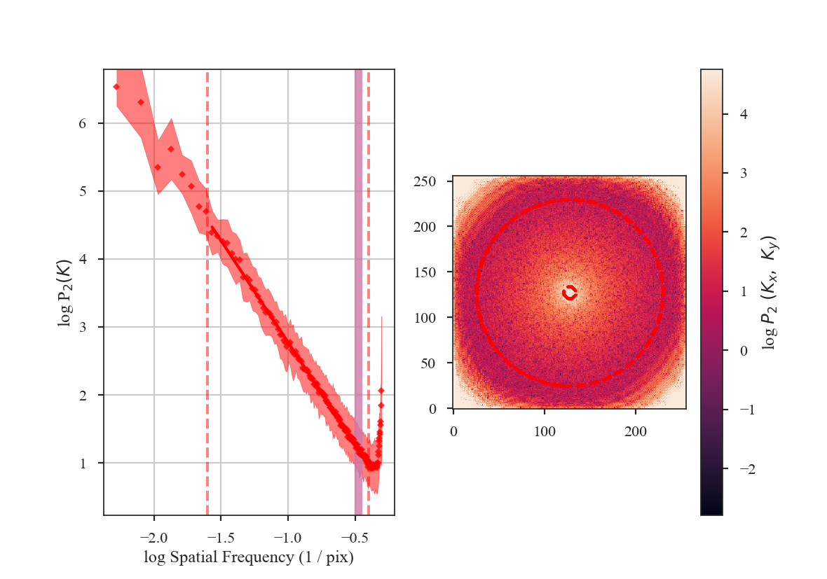
Before exploring the effect of the apodizing kernels, we can demonstrate the need for an apodizing kernel by taking a slice of the red-noise image, such that the edges are no longer periodic.
>>> pspec_partial = PowerSpectrum(rnoise_img[:128, :128], header=plaw_hdu.header).run(verbose=False, fit_2D=False, low_cut=1 / (60. * u.pix))
>>> plt.imshow(np.log10(pspec_partial.ps2D))  # doctest: +SKIP
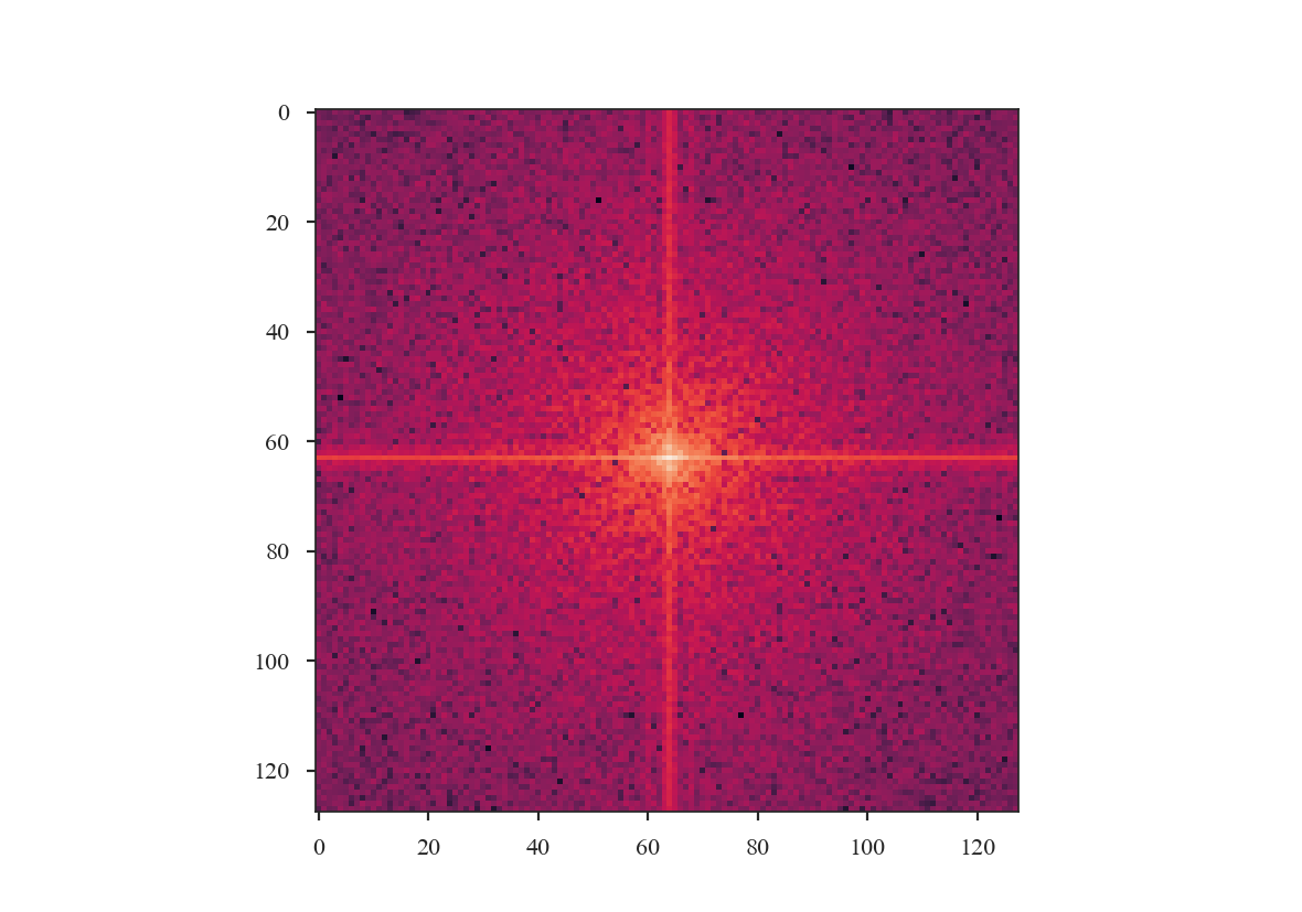
The ringing at large scales is evident in the cross-shape in the 2D power spectrum. This affects the azimuthally-averaged 1D power-spectrum, and therefore the slope of the power-spectrum. Tapering the values at the edges can account for this.
The power-spectrum also appears noisier than the original, yet no noise has been added to the image. This is due to the image no longer being fully sampled for a power-spectrum index of \(3\). This index has most of its power on large scales, so the most prominent structure is on large scales, and slicing has removed significant portions of the large-scale structure. Also note that there is no “hole” at the centre of the 2D power-spectrum since the mean of the sliced image is not \(0\).
We will now compare the how the different apodizing kernels change the power-spectrum shape. The power-spectra will be fit up to scales of \(60\) pixels (or a frequency of \(0.01667\)), avoiding scales that are poorly sampled in the sliced image. The following code computes the power-spectrum of the sliced image using all four of the apodizing kernels shown above.
>>> pspec2 = PowerSpectrum(plaw_hdu)
>>> pspec2.run(verbose=False, radial_pspec_kwargs={'binsize': 1.0},
...            fit_2D=False,
...            low_cut=1. / (60 * u.pix),
...            apodize_kernel='hanning',)  # doctest: +SKIP
>>> pspec3 = PowerSpectrum(plaw_hdu)
>>> pspec3.run(verbose=False, radial_pspec_kwargs={'binsize': 1.0},
...            fit_2D=False,
...            low_cut=1. / (60 * u.pix),
...            apodize_kernel='cosinebell', alpha=0.98)  # doctest: +SKIP
>>> pspec4 = PowerSpectrum(plaw_hdu)
>>> pspec4.run(verbose=False, radial_pspec_kwargs={'binsize': 1.0},
...            fit_2D=False,
...            low_cut=1. / (60 * u.pix),
...            apodize_kernel='splitcosinebell', alpha=0.3, beta=0.8)  # doctest: +SKIP
>>> pspec5 = PowerSpectrum(plaw_hdu)
>>> pspec5.run(verbose=False, radial_pspec_kwargs={'binsize': 1.0},
...            fit_2D=False,
...            low_cut=1. / (60 * u.pix),
...            apodize_kernel='tukey', alpha=0.3)  # doctest: +SKIP
For brevity, we will plot only the 1D power-spectra using the different apodizing kernels.
>>> # Change the colours and comment these lines if you don't use seaborn
>>> import seaborn as sb  # doctest: +SKIP
>>> col_pal = sb.color_palette()  # doctest: +SKIP
>>> pspec.plot_fit(color=col_pal[0], label='Original')  # doctest: +SKIP
>>> pspec2.plot_fit(color=col_pal[1], label='Hanning')  # doctest: +SKIP
>>> pspec3.plot_fit(color=col_pal[2], label='CosineBell')  # doctest: +SKIP
>>> pspec4.plot_fit(color=col_pal[3], label='SplitCosineBell')  # doctest: +SKIP
>>> pspec5.plot_fit(color=col_pal[4], label='Tukey')  # doctest: +SKIP
>>> plt.legend(frameon=True, loc='lower left')  # doctest: +SKIP
>>> plt.ylim([2, 9.5])  # doctest: +SKIP
>>> plt.tight_layout()  # doctest: +SKIP
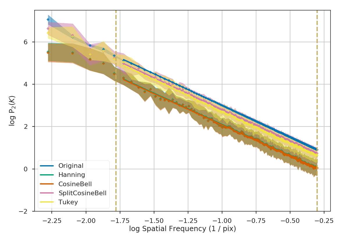
Comparing the different power spectra with different apodizing kernels, the only variations occur on large scales. However, as noted above, the large frequencies suffer from a lack of samples and tend to have underestimated errors. The well-sampled range of frequencies, from 1 to 60 pixels, have a slope that is relatively unaffected regardless of the apodizing kernel that is used. The fitted slopes are:
>>> print("Original: {0:.2f} \nHanning: {1:.2f} \nCosineBell: {2:.2f} \n"
...       "SplitCosineBell: {3:.2f} "
...       "\nTukey: {4:.2f}".format(pspec.slope,
...                                 pspec2.slope,
...                                 pspec3.slope,
...                                 pspec4.slope,
...                                 pspec5.slope))  # doctest: +SKIP
Original: -3.00
Hanning: -2.95
CosineBell: -2.95
SplitCosineBell: -3.00
Tukey: -3.01
Each of the slopes are close to the expected value of \(-3\). The Cosine and Hanning kernels moderately flatten the power-spectra on all scales. This is evident from the figure above comparing the 1D power-spectra of the four kernels.
Warning
The range of frequencies affected by the apodizing kernel depends on the properties of the kernel used. The shape of the kernels are controlled by the \(\alpha\) and/or \(\beta\) parameters (see above). Narrower shapes will tend to have a larger effect on the power-spectrum. It is prudent to check the effect of the apodizing kernel by comparing different choices for the shape!
The optimal choice of apodizing kernel, and the shape parameters for that kernel, will depend on the data that is being used. If there is severe ringing in the power-spectrum, the Hanning or CosineBell kernels are most effective at removing ringing. However, as shown above, these kernels bias the slope at all frequencies. The SplitCosineBell or Tukey are not as affective at removing ringing in extreme cases but they do only bias the shape of the power-spectrum at large frequencies (\(\sim1/2\) of the image size and larger).
Accounting for the beam shape
Warning
The beam size of an observation introduces artificial correlations into the data on scales near to and below the beam size. This affects the shape of various turbulence statistics that measure spatial properties (Spatial Power-Spectrum, MVC, VCA, Delta-Variance, Wavelets, SCF).
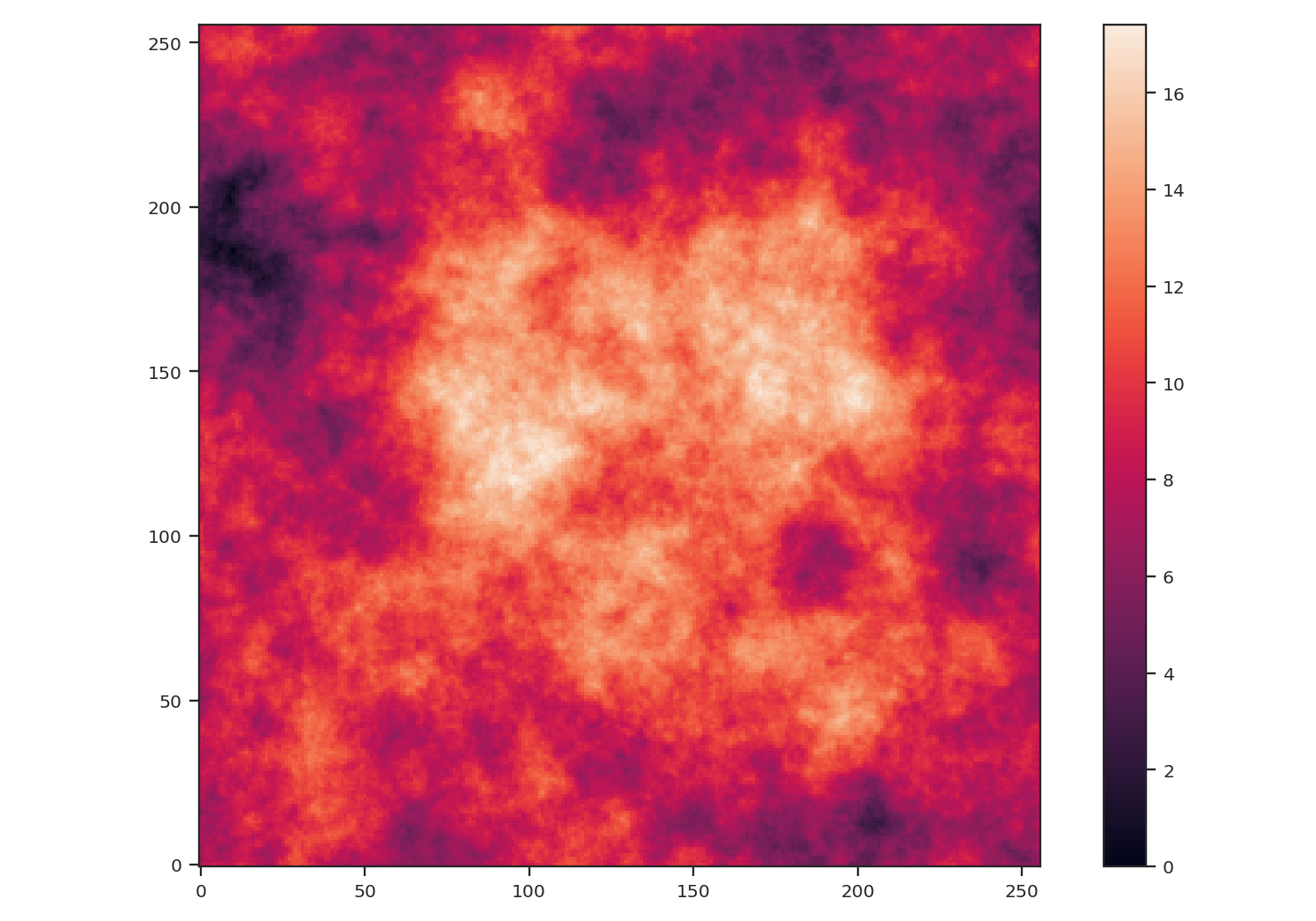
The beam size is typically expressed as the full-width-half-max (FWHM). However, it is important to note that the data will still be correlated beyond the FWHM. For example, consider a randomly-drawn image with a specified power-law index:
>>> import matplotlib.pyplot as plt
>>> from turbustat.simulator import make_extended
>>> from turbustat.io.sim_tools import create_fits_hdu
>>> from astropy import units as u
>>> # Image drawn from red-noise
>>> rnoise_img = make_extended(256, powerlaw=3.)
>>> # Define properties to generate WCS information
>>> pixel_scale = 3 * u.arcsec
>>> beamfwhm = 3 * u.arcsec
>>> imshape = rnoise_img.shape
>>> restfreq = 1.4 * u.GHz
>>> bunit = u.K
>>> # Create a FITS HDU
>>> plaw_hdu = create_fits_hdu(rnoise_img, pixel_scale, beamfwhm, imshape, restfreq, bunit)
>>> plt.imshow(plaw_hdu.data)  # doctest: +SKIP
The power-spectrum of the image should give a slope of 3:
>>> from turbustat.statistics import PowerSpectrum
>>> pspec = PowerSpectrum(plaw_hdu)
>>> pspec.run(verbose=True, radial_pspec_kwargs={'binsize': 1.0},
...           fit_kwargs={'weighted_fit': True}, fit_2D=False,
...           low_cut=1. / (60 * u.pix))  # doctest: +SKIP
                            OLS Regression Results
==============================================================================
Dep. Variable:                      y   R-squared:                       1.000
Model:                            OLS   Adj. R-squared:                  1.000
Method:                 Least Squares   F-statistic:                 8.070e+06
Date:                Thu, 21 Jun 2018   Prob (F-statistic):               0.00
Time:                        11:43:47   Log-Likelihood:                 701.40
No. Observations:                 177   AIC:                            -1399.
Df Residuals:                     175   BIC:                            -1392.
Df Model:                           1
Covariance Type:            nonrobust
==============================================================================
                 coef    std err          t      P>|t|      [0.025      0.975]
------------------------------------------------------------------------------
const          0.0032      0.001      3.952      0.000       0.002       0.005
x1            -2.9946      0.001  -2840.850      0.000      -2.997      -2.992
==============================================================================
Omnibus:                      252.943   Durbin-Watson:                   1.077
Prob(Omnibus):                  0.000   Jarque-Bera (JB):            26797.433
Skew:                          -5.963   Prob(JB):                         0.00
Kurtosis:                      62.087   Cond. No.                         4.55
==============================================================================
Now we will smooth this image with a Gaussian beam. The easiest way to do this is to use the built-in
tools from the spectral-cube and
radio_beam packages.
We will convert the FITS HDU to a spectral-cube Projection, and define a pencil beam for the
initial image:
>>> from spectral_cube import Projection
>>> from radio_beam import Beam
>>> pencil_beam = Beam(0 * u.deg)
>>> plaw_proj = Projection.from_hdu(plaw_hdu)
>>> plaw_proj = plaw_proj.with_beam(pencil_beam)
Next we will define the beam to smooth to. A 3-pixel wide FWHM is reasonable:
>>> new_beam = Beam(3 * plaw_hdu.header['CDELT2'] * u.deg)
>>> plaw_conv = plaw_proj.convolve_to(new_beam)
>>> plaw_conv.quicklook()  # doctest: +SKIP
How has smoothing changed the shape of the power-spectrum?
>>> # Change the colours and comment these lines if you don't use seaborn
>>> import seaborn as sb  # doctest: +SKIP
>>> col_pal = sb.color_palette()  # doctest: +SKIP
>>> pspec2 = PowerSpectrum(plaw_conv)
>>> pspec2.run(verbose=True, xunit=u.pix**-1, fit_2D=False,
...            low_cut=0.025 / u.pix, high_cut=0.1 / u.pix,
...            radial_pspec_kwargs={'binsize': 1.0},
...            apodize_kernel='tukey')  # doctest: +SKIP
>>> plt.axvline(np.log10(1 / 3.), color=col_pal[3], linewidth=8, alpha=0.8,
...             zorder=1)  # doctest: +SKIP
                            OLS Regression Results
==============================================================================
Dep. Variable:                      y   R-squared:                       0.988
Model:                            OLS   Adj. R-squared:                  0.988
Method:                 Least Squares   F-statistic:                     2059.
Date:                Thu, 21 Jun 2018   Prob (F-statistic):           1.54e-25
Time:                        14:23:19   Log-Likelihood:                 35.997
No. Observations:                  27   AIC:                            -67.99
Df Residuals:                      25   BIC:                            -65.40
Df Model:                           1
Covariance Type:            nonrobust
==============================================================================
                 coef    std err          t      P>|t|      [0.025      0.975]
------------------------------------------------------------------------------
const         -1.0626      0.098    -10.848      0.000      -1.264      -0.861
x1            -3.5767      0.079    -45.378      0.000      -3.739      -3.414
==============================================================================
Omnibus:                        3.417   Durbin-Watson:                   0.840
Prob(Omnibus):                  0.181   Jarque-Bera (JB):                2.072
Skew:                          -0.650   Prob(JB):                        0.355
Kurtosis:                       3.391   Cond. No.                         15.7
==============================================================================
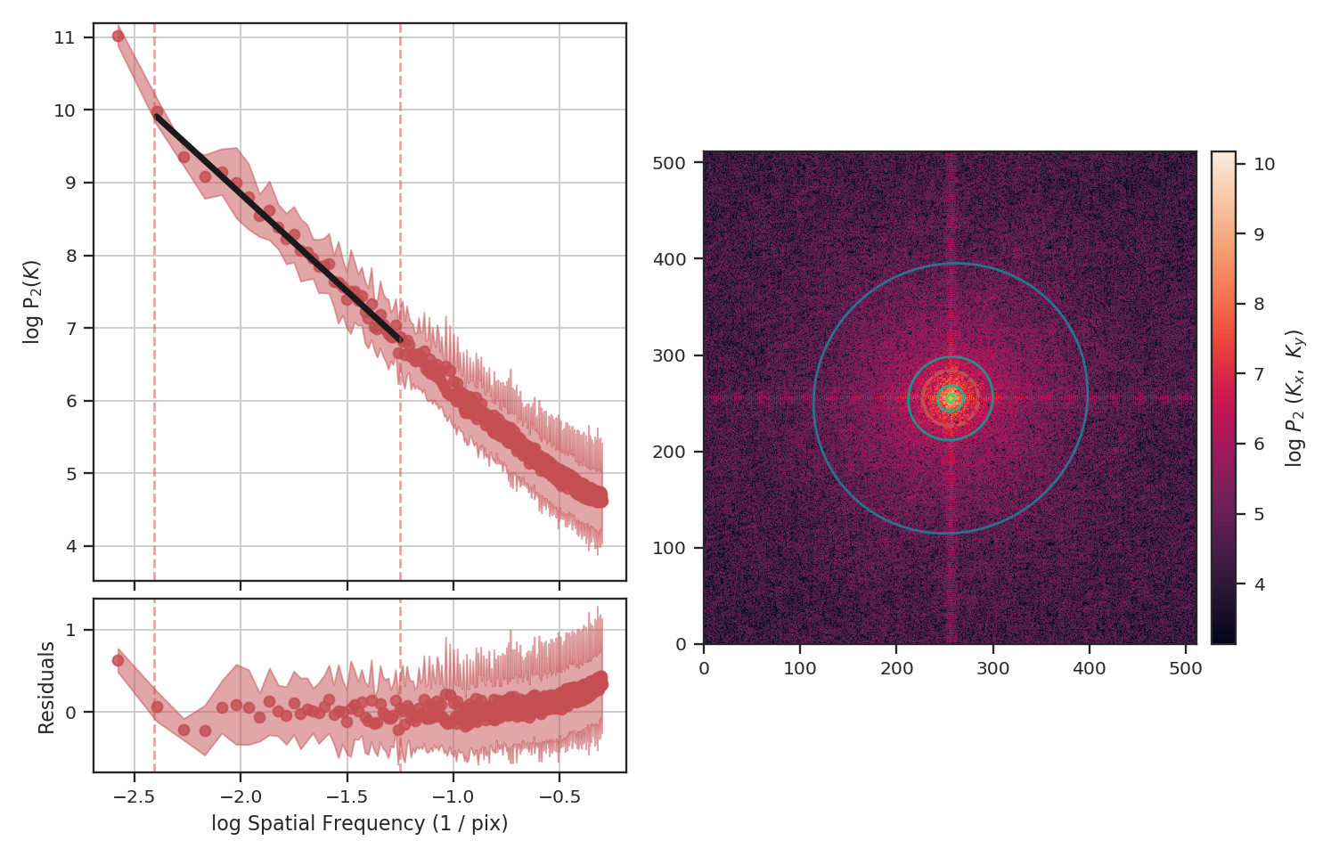
The slope of the power-spectrum is significantly steepened on small scales by the beam (see the reported result in variable x1 above).
And this steepening occurs on scales much larger than the beam FWHM, which is indicated by
the thick purple vertical line in the left-hand side of the plot. The fitting was restricted to scales much larger than three times the beam width. However, the recovered slope is still steeper than the original -3.
Also note that convolving the image with the beam causes some tapering at the edges of the image, breaking the periodicity at the edges. The image was apodized with a Tukey window, which causes some of the deviations at large scales (small frequencies). See the tutorial page on apodizing kernels for more.
The beam size must be corrected for in the image prior to fitting the power-spectrum. This can be done by (1) including a Gaussian beam component in the model used to fit the power-spectrum, or (2) divide the power-spectrum of the image by the power-spectrum of the beam response. The former requires using a non-linear model, and is not currently implemented in TurbuStat (see Martin et al. 2015 for an example). The latter method can be applied prior to fitting, allowing a linear model to still be used for fitting.
The beam correction in TurbuStat requires the optional package radio_beam to be installed. radio_beam allows the beam response for any 2D elliptical Gaussian to be returned. For statistics that create a power-spectrum (Spatial Power-Spectrum, VCA, MVC), the beam correction can be applied by specifying beam_correct=True:
>>> pspec3 = PowerSpectrum(plaw_conv)
>>> pspec3.run(verbose=True, xunit=u.pix**-1, fit_2D=False,
...            low_cut=0.025 / u.pix, high_cut=0.4 / u.pix,
...            apodize_kernel='tukey', beam_correct=True)  # doctest: +SKIP
>>> plt.axvline(np.log10(1 / 3.), color=col_pal[3], linewidth=8, alpha=0.8,
...             zorder=1)  # doctest: +SKIP
                            OLS Regression Results
==============================================================================
Dep. Variable:                      y   R-squared:                       0.998
Model:                            OLS   Adj. R-squared:                  0.998
Method:                 Least Squares   F-statistic:                 8.828e+04
Date:                Thu, 21 Jun 2018   Prob (F-statistic):          5.55e-192
Time:                        14:38:33   Log-Likelihood:                 268.87
No. Observations:                 137   AIC:                            -533.7
Df Residuals:                     135   BIC:                            -527.9
Df Model:                           1
Covariance Type:            nonrobust
==============================================================================
                 coef    std err          t      P>|t|      [0.025      0.975]
------------------------------------------------------------------------------
const         -0.2247      0.008    -27.671      0.000      -0.241      -0.209
x1            -2.9961      0.010   -297.116      0.000      -3.016      -2.976
==============================================================================
Omnibus:                        7.089   Durbin-Watson:                   1.500
Prob(Omnibus):                  0.029   Jarque-Bera (JB):                9.274
Skew:                           0.285   Prob(JB):                      0.00969
Kurtosis:                       4.140   Cond. No.                         5.50
==============================================================================
The shape of the power-spectrum has been restored and we recover the correct slope. The deviation on small scales (large frequencies) occurs on scales smaller than about the FWHM of the beam where the information has been lost by the spatial smoothing applied to the image. If the beam is over-sampled by a larger factor — say with a 6-pixel FWHM instead of 3 — the increase in power on small scales will affect a larger region of the power-spectrum. This region should be excluded from the power-spectrum fit. A reasonable lower-limit to fit the power-spectrum to is the FWHM of the beam. Additional noise in the image will tend to flatten the power-spectrum to larger scales, so setting the lower fitting limit to a couple times the beam width may be necessary. We recommend visually examining the quality of the fit.
Here are the three power-spectra shown above overplotted to highlight the shape changes from spatial smoothing:
>>> pspec.plot_fit(color=col_pal[0], label='Original')  # doctest: +SKIP
>>> pspec2.plot_fit(color=col_pal[1], label='Smoothed')  # doctest: +SKIP
>>> pspec3.plot_fit(color=col_pal[2], label='Beam-Corrected')  # doctest: +SKIP
>>> plt.legend(frameon=True, loc='lower left')  # doctest: +SKIP
>>> plt.axvline(np.log10(1 / 3.), color=col_pal[3], linewidth=8, alpha=0.8, zorder=-1)  # doctest: +SKIP
>>> plt.ylim([-2, 7.5])  # doctest: +SKIP
>>> plt.tight_layout()  # doctest: +SKIP
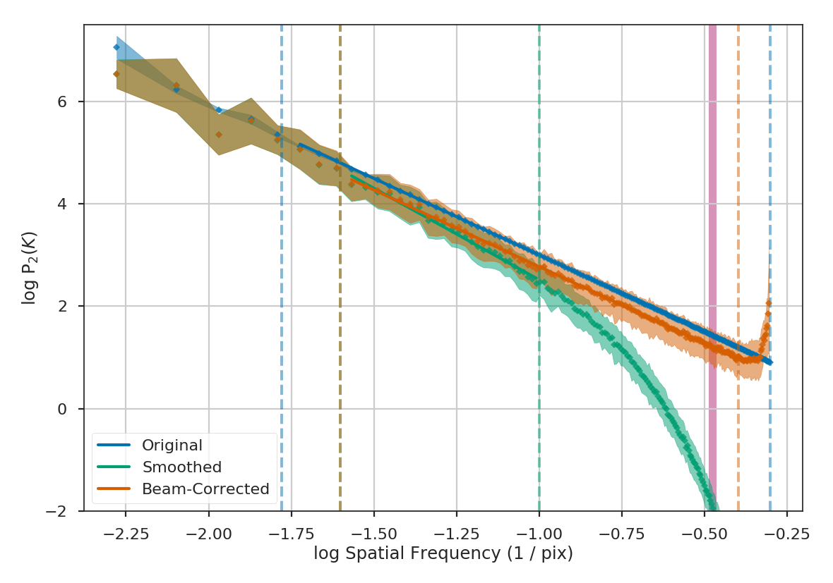
Similar fitting restrictions apply to the MVC and VCA, as well. The beam correction can be applied in the same manner as described above. For other spatial methods which do not use the power-spectrum, the scales of the beam should at least be excluded from any fitting. For example, lag scales smaller than the beam in the Delta-Variance, Wavelets, and SCF should not be fit. The spatial filtering used to measure Statistical Moments should be set to a width of at least the beam size.
Dealing with missing data
When running any statistic in TurbuStat on data set with noise, there is a question of whether or not to mask out noisy data. Masking noisy data is a common practice with observational data and is often crucial for recovering scientifically-usable results. However, some of the statistics in TurbuStat implicitly assume the map is continuous. This page demonstrates the pros and cons of masking data versus including noisy regions.
We will create a red noise image to use as an example:
>>> import numpy as np
>>> import matplotlib.pyplot as plt
>>> from turbustat.simulator import make_extended
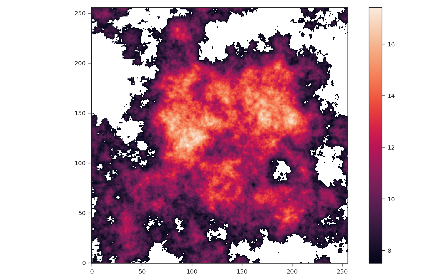
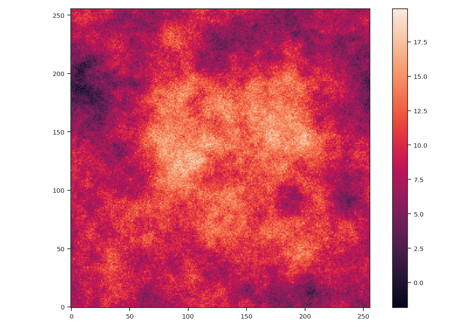
>>> img = make_extended(256, powerlaw=3., randomseed=54398493)
>>> # Now shuffle so the peak is near the centre
>>> img = np.roll(img, (128, -30), (0, 1))
>>> img -= img.min()
>>> plt.imshow(img, origin='lower')
>>> plt.colorbar()
After creating the image, we centered the peak of the map to be near the centre. We also subtracted the minimum value from the image to remove negative values to better mimic observational data.
We will compare the effect of noise and masking on two statistics: the PowerSpectrum and the Delta-variance. The power-spectrum relies on a Fast Fourier Transform (FFT), which implicitly assumes that the map edges are periodic. This assumption presents an issue for observational maps with emission at their edge and requires an apodizing kernel to be applied to the data prior to computing the power-spectrum. The delta-variance relies on convolving the map by a set of kernels with increasing size. While the convolution also uses a Fourier transform, noisy or missing regions in the data are down-weighted so this method can be used on observational data with arbitrary shape (Ossenkopf at al. 2008a).
Note
Throughout this example, we will not create realistic WCS information for the image because we will be altering the image in each step. For brevity, we pass fits.PrimaryHDU(img) which creates a FITS HDU without complete WCS information. For a tutorial on how TurbuStat creates mock WCS information, see here.
First, we will use both statistics on the unaltered image:
>>> from astropy.io import fits
>>> from turbustat.statistics import PowerSpectrum, DeltaVariance
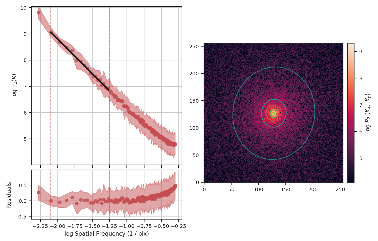
>>> pspec = PowerSpectrum(fits.PrimaryHDU(img))
>>> pspec.run(verbose=True)
OLS Regression Results
==============================================================================
Dep. Variable: y R-squared: 1.000
Model: OLS Adj. R-squared: 1.000
Method: Least Squares F-statistic: 3.239e+05
Date: Thu, 14 Feb 2019 Prob (F-statistic): 1.61e-293
Time: 17:08:19 Log-Likelihood: 610.32
No. Observations: 181 AIC: -1217.
Df Residuals: 179 BIC: -1210.
Df Model: 1
Covariance Type: HC3
==============================================================================
coef std err z P>|z| [0.025 0.975]
------------------------------------------------------------------------------
const 2.3594 0.003 755.971 0.000 2.353 2.366
x1 -2.9893 0.005 -569.096 0.000 -3.000 -2.979
==============================================================================
Omnibus: 150.694 Durbin-Watson: 1.634
Prob(Omnibus): 0.000 Jarque-Bera (JB): 5853.912
Skew: -2.593 Prob(JB): 0.00
Kurtosis: 30.374 Cond. No. 4.15
==============================================================================
The power-spectrum recovers the expected slope of \(-3\). The delta-variance slope should be \(-\beta -2\), where \(\beta\) is the power-spectrum slope, so we should find a slope of \(1\):
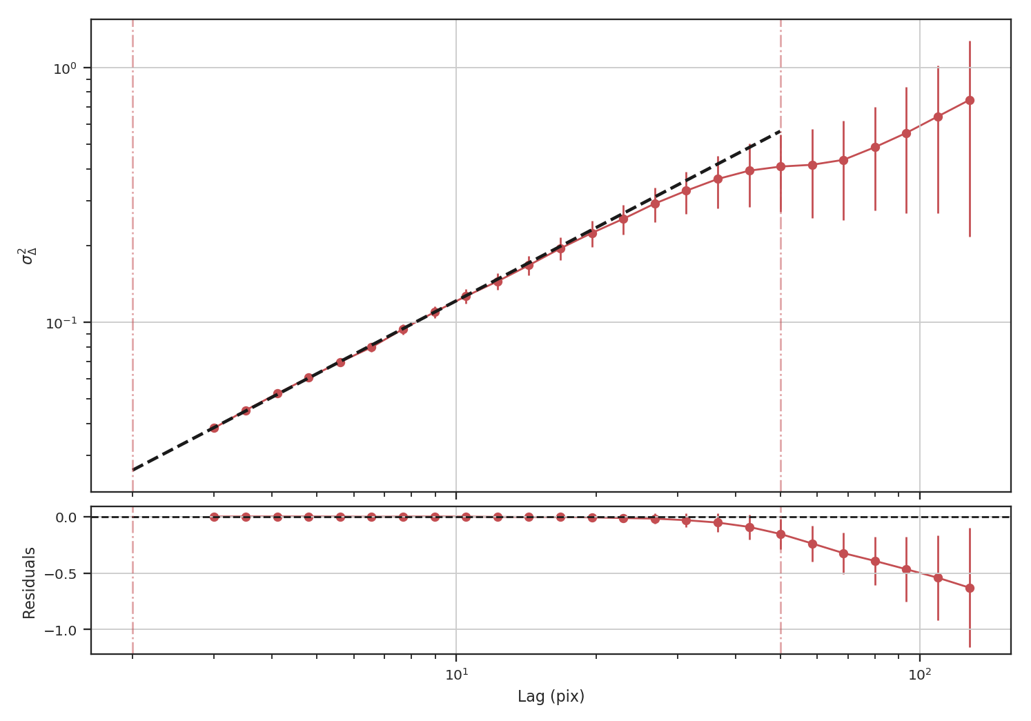
>>> delvar = DeltaVariance(fits.PrimaryHDU(img))
>>> delvar.run(verbose=True)
                       WLS Regression Results
==============================================================================
Dep. Variable:                      y   R-squared:                       0.999
Model:                            WLS   Adj. R-squared:                  0.999
Method:                 Least Squares   F-statistic:                     1741.
Date:                Thu, 14 Feb 2019   Prob (F-statistic):           3.50e-23
Time:                        17:13:16   Log-Likelihood:                 48.412
No. Observations:                  25   AIC:                            -92.82
Df Residuals:                      23   BIC:                            -90.39
Df Model:                           1
Covariance Type:                  HC3
==============================================================================
                 coef    std err          z      P>|z|      [0.025      0.975]
------------------------------------------------------------------------------
const         -1.8780      0.017   -113.441      0.000      -1.910      -1.846
x1             0.9986      0.024     41.723      0.000       0.952       1.046
==============================================================================
Omnibus:                        6.913   Durbin-Watson:                   1.306
Prob(Omnibus):                  0.032   Jarque-Bera (JB):                6.334
Skew:                           0.535   Prob(JB):                       0.0421
Kurtosis:                       5.221   Cond. No.                         12.1
==============================================================================
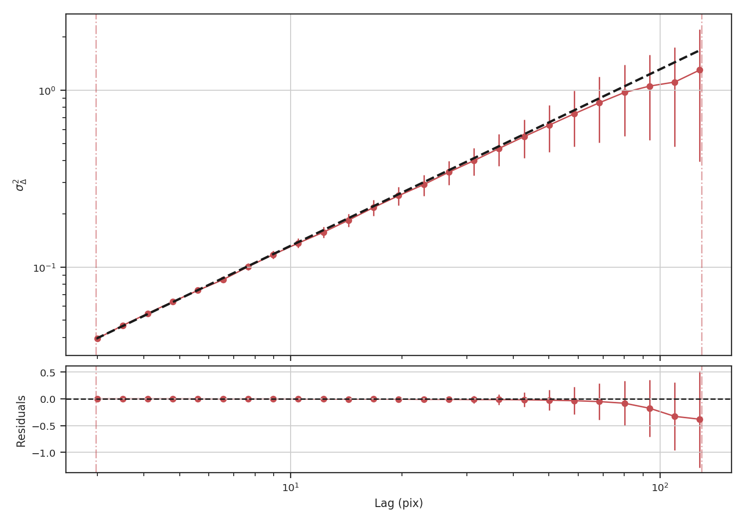
Indeed, we recover the correct slope from the delta-variance.
To demonstrate how masking affects each of these statistics, we will arbitrarily mask low values below the 25 percentile in the example image and run each statistic:
>>> masked_img = img.copy()
>>> masked_img[masked_img < np.percentile(img, 25)] = np.NaN
>>> plt.imshow(masked_img, origin='lower')
>>> plt.colorbar()
The central bright region remains but much of the fainter features around the image edges have been masked.:
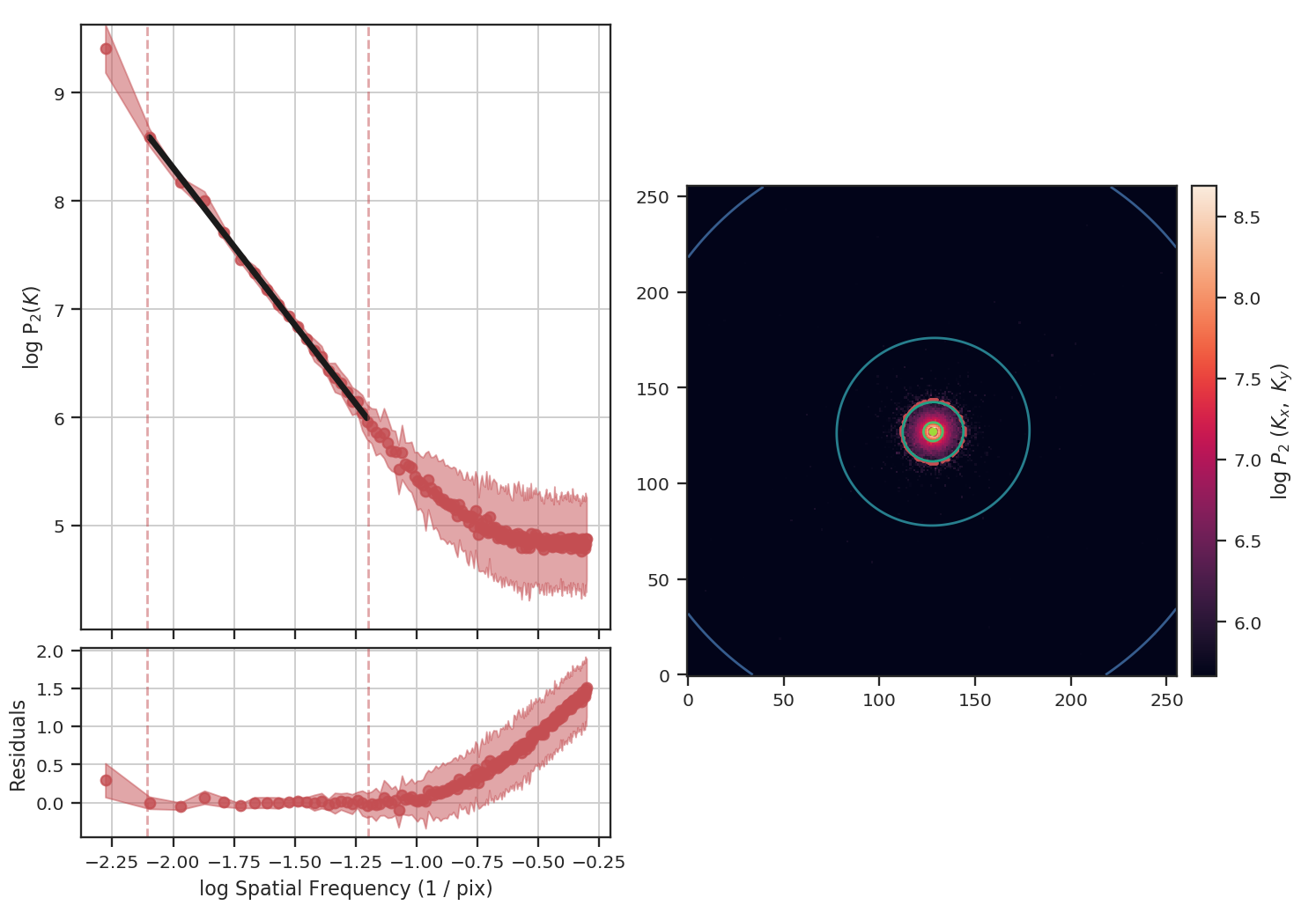
>>> pspec_masked = PowerSpectrum(fits.PrimaryHDU(masked_img))
>>> pspec_masked.run(verbose=True, high_cut=10**-1.25 / u.pix)
                            OLS Regression Results
==============================================================================
Dep. Variable:                      y   R-squared:                       0.993
Model:                            OLS   Adj. R-squared:                  0.993
Method:                 Least Squares   F-statistic:                     2636.
Date:                Thu, 14 Feb 2019   Prob (F-statistic):           3.45e-19
Time:                        17:19:21   Log-Likelihood:                 27.859
No. Observations:                  18   AIC:                            -51.72
Df Residuals:                      16   BIC:                            -49.94
Df Model:                           1
Covariance Type:                  HC3
==============================================================================
                 coef    std err          z      P>|z|      [0.025      0.975]
------------------------------------------------------------------------------
const          3.5321      0.080     44.347      0.000       3.376       3.688
x1            -2.6362      0.051    -51.344      0.000      -2.737      -2.536
==============================================================================
Omnibus:                        0.336   Durbin-Watson:                   2.692
Prob(Omnibus):                  0.845   Jarque-Bera (JB):                0.445
Skew:                           0.259   Prob(JB):                        0.800
Kurtosis:                       2.429   Cond. No.                         14.6
==============================================================================
Masking has significantly flattened the power-spectrum, even with the restriction we added to fit only scales larger than \(10^{1.25}\sim18\) pixels. In fact, flattening the power-spectrum is similar to how noise effects the power-spectrum. Why is this? FFTs cannot be used on data with missing values specified as NaNs. Instead, we have to choose a finite value to _fill_ the missing data; we typically choose to fill these regions with \(0\). When large regions are missing, the fill value leads to a large region with constant values that, by itself, would have a power-spectrum index of \(0\).
The delta-variance avoids the filling issue for masked data by introducing weights. Places with missing data have a very low weight or remained masked. The astropy convolution package has routines for interpolating over masked data, which is useful when small regions are missing data but is not typically useful when the missing data lies at the edge of emission in a map. With the masked image, the delta-variance curve we find is:
>>> delvar_masked = DeltaVariance(fits.PrimaryHDU(masked_img))
>>> delvar_masked.run(verbose=True, xlow=2 * u.pix, xhigh=50 * u.pix)
                            WLS Regression Results
==============================================================================
Dep. Variable:                      y   R-squared:                       0.999
Model:                            WLS   Adj. R-squared:                  0.999
Method:                 Least Squares   F-statistic:                     1860.
Date:                Thu, 14 Feb 2019   Prob (F-statistic):           5.52e-18
Time:                        17:30:29   Log-Likelihood:                 52.504
No. Observations:                  18   AIC:                            -101.0
Df Residuals:                      16   BIC:                            -99.23
Df Model:                           1
Covariance Type:                  HC3
==============================================================================
                 coef    std err          z      P>|z|      [0.025      0.975]
------------------------------------------------------------------------------
const         -1.8679      0.015   -120.680      0.000      -1.898      -1.838
x1             0.9520      0.022     43.128      0.000       0.909       0.995
==============================================================================
Omnibus:                        4.484   Durbin-Watson:                   1.339
Prob(Omnibus):                  0.106   Jarque-Bera (JB):                2.180
Skew:                           0.694   Prob(JB):                        0.336
Kurtosis:                       3.991   Cond. No.                         11.7
==============================================================================
When restricting the fit to scales of less than 50 pixels (about a quarter of the image), we recover a slope of \(0.95\), significantly closer to the expected value of \(1.0\) relative to the power-spectrum.
Another issue that could be encountered with observational data are large empty regions in a map, either due to masking (similar to the above example) or when we want to investigate a single object and have masked out all others. This situation could arise when the data are segmented into individual _”blobs”_ and we want to study the properties of each blob. To mimic this situation, we will pad the edges (following the numpy example) of the image with empty values as:
>>> def pad_with(vector, pad_width, iaxis, kwargs):
... pad_value = kwargs.get('padder', 0.)
... vector[:pad_width[0]] = pad_value
... vector[-pad_width[1]:] = pad_value
... return vector
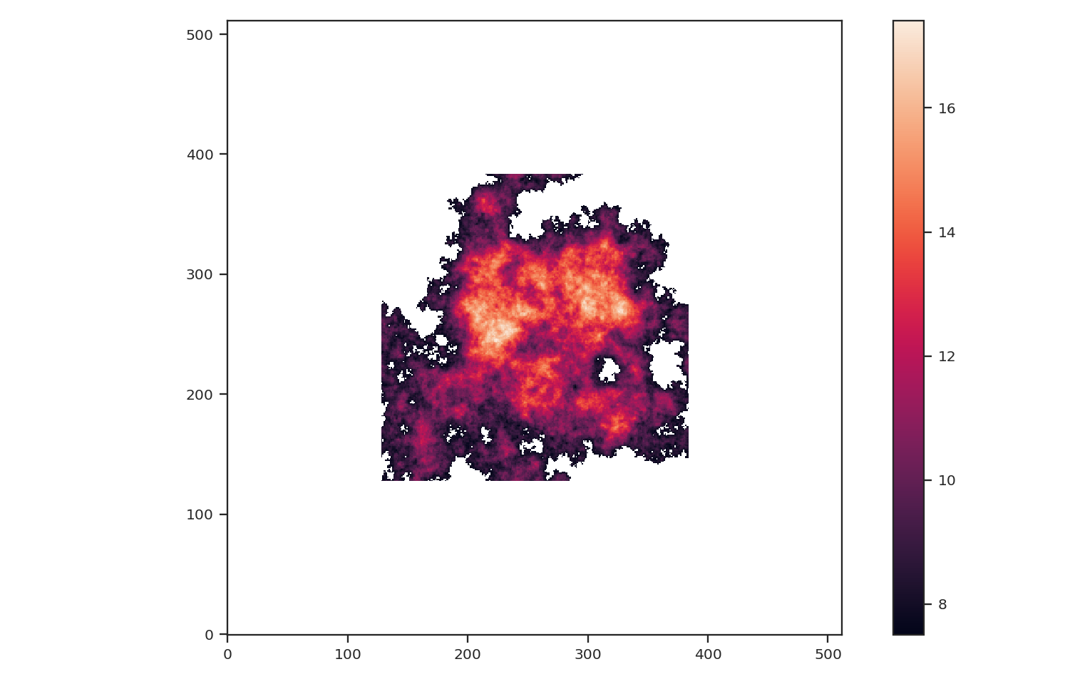
>>> padded_masked_img = np.pad(masked_img, 128, pad_with, padder=np.NaN)
We are also only going to keep the biggest continuous region in the padded image to mimic studying a single object picked from a larger image:
>>> from scipy import ndimage as nd
>>> labs, num = nd.label(np.isfinite(padded_masked_img), np.ones((3, 3)))
>>> # Keep the largest region only
>>> padded_masked_img[np.where(labs > 1)] = np.NaN
>>> plt.imshow(padded_masked_img, origin='lower')
>>> plt.colorbar()
The unmasked region is now surrounded by huge empty regions. How does this affect the power-spectrum and delta-variance?:
>>> pspec_masked_pad = PowerSpectrum(fits.PrimaryHDU(padded_masked_img))
>>> pspec_masked_pad.run(verbose=True, high_cut=10**-1.25 / u.pix)

                            OLS Regression Results
==============================================================================
Dep. Variable:                      y   R-squared:                       0.985
Model:                            OLS   Adj. R-squared:                  0.985
Method:                 Least Squares   F-statistic:                     1166.
Date:                Fri, 15 Feb 2019   Prob (F-statistic):           1.41e-29
Time:                        13:43:42   Log-Likelihood:                 35.094
No. Observations:                  39   AIC:                            -66.19
Df Residuals:                      37   BIC:                            -62.86
Df Model:                           1
Covariance Type:                  HC3
==============================================================================
                 coef    std err          z      P>|z|      [0.025      0.975]
------------------------------------------------------------------------------
const          3.4746      0.123     28.245      0.000       3.233       3.716
x1            -2.6847      0.079    -34.144      0.000      -2.839      -2.531
==============================================================================
Omnibus:                        1.962   Durbin-Watson:                   2.222
Prob(Omnibus):                  0.375   Jarque-Bera (JB):                1.840
Skew:                          -0.489   Prob(JB):                        0.399
Kurtosis:                       2.580   Cond. No.                         12.2
==============================================================================
The power-spectrum is similarly flattened as in the non-padded case. However, the sharp cut-off at the edges of the non-masked region lead to the Gibbs phenomenon (i.e., ringing) evident from the horizontal and vertical stripes in the 2D power-spectrum on the right. The ringing can be minimized by utilizing an apodizing kernel.
>>> delvar_masked_padded = DeltaVariance(fits.PrimaryHDU(padded_masked_img))
>>> delvar_masked_padded.run(verbose=True, xlow=2 * u.pix, xhigh=70 * u.pix)  # doctest: +SKIP
                            WLS Regression Results
==============================================================================
Dep. Variable:                      y   R-squared:                       0.999
Model:                            WLS   Adj. R-squared:                  0.999
Method:                 Least Squares   F-statistic:                 1.120e+04
Date:                Fri, 15 Feb 2019   Prob (F-statistic):           3.37e-24
Time:                        13:48:37   Log-Likelihood:                 48.777
No. Observations:                  18   AIC:                            -93.55
Df Residuals:                      16   BIC:                            -91.77
Df Model:                           1
Covariance Type:                  HC3
==============================================================================
                 coef    std err          z      P>|z|      [0.025      0.975]
------------------------------------------------------------------------------
const         -1.8663      0.004   -425.902      0.000      -1.875      -1.858
x1             0.9501      0.009    105.823      0.000       0.933       0.968
==============================================================================
Omnibus:                       26.283   Durbin-Watson:                   1.593
Prob(Omnibus):                  0.000   Jarque-Bera (JB):               41.814
Skew:                          -2.253   Prob(JB):                     8.32e-10
Kurtosis:                       8.953   Cond. No.                         11.6
==============================================================================
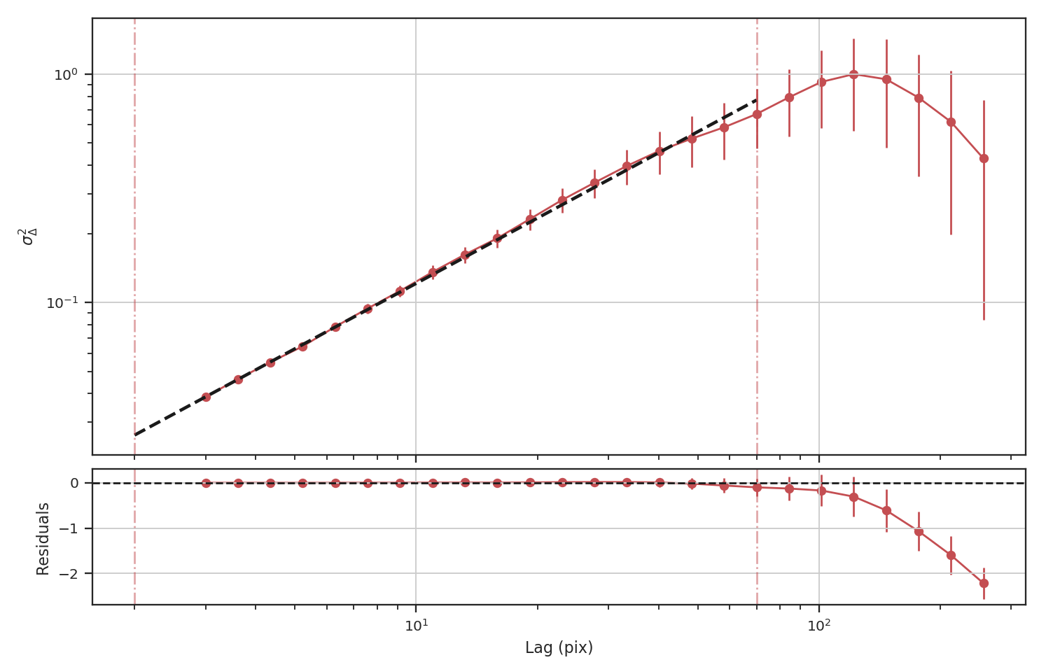
The delta-variance is similarly unaffected by the padded region. Because of the weighting functions, the convolution steps in the delta-variance do not suffer from ringing like the power-spectrum does. We note that this delta-variance curve extends to larger scales because of the padding. What is notable on these larger scales is the lack of emission, which causes the delta-variance to decrease. This is the expected behaviour when large regions of an image are masked and the user can either (i) limit the lags to smaller values, or (ii) exclude large scales from the fit (as we do in this example).
Now, we will compare the masking examples above to when noise is added to the image (without padding). We will add noise to the image drawn from a normal distribution with standard deviation of 1.:
>>> noise_rms = 1.
>>> noisy_img = img + np.random.normal(0., noise_rms, img.shape)
>>> plt.imshow(noisy_img, origin='lower')
>>> plt.colorbar()
Since the noise distribution is spatially-uncorrelated, the power-spectrum of only the noise will be 0. We expect then that the power-spectrum will be flattened on small scales due to the noise:
>>> pspec_noisy = PowerSpectrum(fits.PrimaryHDU(noisy_img))
>>> pspec_noisy.run(verbose=True, high_cut=10**-1.2 / u.pix)
                            OLS Regression Results
==============================================================================
Dep. Variable:                      y   R-squared:                       0.999
Model:                            OLS   Adj. R-squared:                  0.999
Method:                 Least Squares   F-statistic:                     7447.
Date:                Fri, 15 Feb 2019   Prob (F-statistic):           4.08e-26
Time:                        13:58:28   Log-Likelihood:                 47.231
No. Observations:                  21   AIC:                            -90.46
Df Residuals:                      19   BIC:                            -88.37
Df Model:                           1
Covariance Type:                  HC3
==============================================================================
                 coef    std err          z      P>|z|      [0.025      0.975]
------------------------------------------------------------------------------
const          2.4964      0.048     51.948      0.000       2.402       2.591
x1            -2.9054      0.034    -86.298      0.000      -2.971      -2.839
==============================================================================
Omnibus:                        3.284   Durbin-Watson:                   2.477
Prob(Omnibus):                  0.194   Jarque-Bera (JB):                1.493
Skew:                           0.450   Prob(JB):                        0.474
Kurtosis:                       3.948   Cond. No.                         13.3
==============================================================================
The power-spectrum does indeed approach an index of 0 on small scales due to the noise. By excluding scales smaller than \(10^{1.25}\sim18\) pixels, however, we recover a index of \(-2.9\), much closer to the actual index of \(-3\) than the masking example above. The extent that the power-spectrum index will be biased by the noise will depend on the level of noise relative to the signal. An alternative approach to model the power-spectrum would be to include a noise component (e.g., Miville-Deschenes et al. 2010) but this is not currently implemented in TurbuStat.
Running delta-variance on the noisy image gives:
>>> delvar_noisy = DeltaVariance(fits.PrimaryHDU(noisy_img))
>>> delvar_noisy.run(verbose=True, xlow=10 * u.pix, xhigh=70 * u.pix)
                            WLS Regression Results
==============================================================================
Dep. Variable:                      y   R-squared:                       0.999
Model:                            WLS   Adj. R-squared:                  0.998
Method:                 Least Squares   F-statistic:                     842.9
Date:                Fri, 15 Feb 2019   Prob (F-statistic):           9.52e-12
Time:                        14:17:20   Log-Likelihood:                 41.456
No. Observations:                  13   AIC:                            -78.91
Df Residuals:                      11   BIC:                            -77.78
Df Model:                           1
Covariance Type:                  HC3
==============================================================================
                 coef    std err          z      P>|z|      [0.025      0.975]
------------------------------------------------------------------------------
const         -1.8245      0.041    -45.005      0.000      -1.904      -1.745
x1             0.9480      0.033     29.034      0.000       0.884       1.012
==============================================================================
Omnibus:                        7.660   Durbin-Watson:                   1.670
Prob(Omnibus):                  0.022   Jarque-Bera (JB):                3.768
Skew:                          -1.137   Prob(JB):                        0.152
Kurtosis:                       4.336   Cond. No.                         20.7
==============================================================================
The delta-variance slope is flatter by about the same amount as in the masked image example above (\(0.95\)). Thus masking and noise (at this level) have the same effect on the slope of the delta-variance.
From these examples, we see that the power-spectrum is more biased by masking than by keeping noisy regions in the image. The delta-variance is similarly biased in both cases because of how noisy regions are down-weighted in the convolution step.
Note
We encourage users to test a statistic with and without masking their data to determine how the statistic is affected by masking.
Where noise matters
Noise will affect all the statistics and metrics in TurbuStat to some extent. This section lists common issues that may be encountered with observational data.
- The previous section shows an example of how noise flattens a power-spectrum. This will effect the spatial power-spectrum, MVC, VCA, VCS (at small scales), the Wavelet transform, and the delta-variance. If the noise level is moderate, the range that is fit can be altered to avoid the scales where noise severely flattens the power-spectrum or equivalent relation.
- Fits to the PDF can be affected by noise. These values will tend to cluster the low values in an image to around 0. If the noise is (mostly) uncorrelated, the noise component will be a Gaussian. A minimum value to include in the PDF should be set to avoid this region. Furthermore, the default log-normal model cannot handle negative values and will raise an error in this case.
- Many of the distance metrics are defined in terms of the significance of the difference between two values. For example, the power-spectrum distance is the absolute difference between two indices normalized by the square root of the sum of the variance from the fit uncertainty (\(d=|\beta_1 - \beta_2|\, /\, \sqrt{\sigma_1^2 + \sigma_2^2}\)). If one data set is significantly noisier than the other, this will _lower_ the distance. It is important to compare all distance to a common baseline. This will determine the significance of a distance rather than its value. Koch et al. 2017 explore this in detail.
Statistics
Using statistics classes
The statistics implemented in TurbuStat are python classes. This structure allows for derived properties to persist without having to manually carry them forward through each step.
Using most of the statistic classes will involved two steps:
Initialization – The data, relevant WCS information, and other unchanging properties (like the distance) are specified here. Some of the statistics calculated at specific scales (like
WaveletorSCF) can have those scales set here, too. Below is an example usingWavelet:>>> from turbustat.statistics import Wavelet >>> import numpy as np >>> from astropy.io import fits >>> from astropy.units import u >>> hdu = fits.open("file.fits")[0] # doctest: +SKIP >>> spatial_scales = np.linspace(0.1, 1.0, 20) * u.pc # doctest: +SKIP >>> wave = Wavelet(hdu, scales=spatial_scales, ... distance=260 * u.pc) # doctest: +SKIP
The run function – For most use-cases, the
runfunction can be used to compute the statistic. All of the statistics have this function. It will compute the statistic, perform any relevant fitting, and optionally create a summary plot. The docstring for each of therunfunctions describe the parameters that can be changed from this function. The parameters that are critical to the behaviour of the statistic can all be set fromrun. Continuing with theWaveletexample from above, therunfunction is called as:>>> wave.run(verbose=True, xlow=0.2 * u.pc, xhigh=0.8 * u.pc) # doctest: +SKIP
This function will run the wavelet transform and fit the relation between the given bounds (xlow and xhigh). With verbose=True, a summary plot is returned.
What if you need to set parameters not accessible from run? run wraps multiple steps in one function, however, the statistic can be run in steps when fine-tuning is needed for a particular data set. Each of the statistics has at least one computational step. For Wavelet, there are two steps: (1) computing the transform (compute_transform) and (2) fitting the log of the transform (fit_transform). Running these two functions is equivalent to using run.
The statistics also have plotting functions. From run, these functions are called whenever verbose=True is given. All of the plotting functions start with plot_; for Wavelet, the plotting function is plot_transform. Supplying a save_name to this function will save the figure, the x-units can also be set for spatial transforms (like the wavelet transform) as pixel, angular, or physical (when a distance is given) units, and additional arguments can be given to set the colours and markers used in the plot.
Statistic classes can also be saved or loaded as pickle files. Saving is performed with the save_results function:
>>> wave.save_results("wave_file.pkl", keep_data=False) # doctest: +SKIP
Whether to include the data in saved file is set with keep_data. By default, the data is not saved to save storage space.
Note
If the statistic is not saved with the data, it cannot be recomputed after loading.
Loading the statistic from a saved file uses the load_results function:
>>> new_wave = Wavelet.load_results("wav_file.pkl") # doctest: +SKIP
Unless the data is saved, everything but the data is new accessible from new_wave.
Bispectrum
Overview
The bispectrum is the Fourier transform of the three-point covariance function. It represents the next higher-order expansion upon the more commonly-used two-point statistics, where the autocorrelation function is the Fourier transform of the power spectrum. The bispectrum is computed using:
where \(\ast\) denotes the complex conjugate, \(F\) is the Fourier transform of some signal, and \(k_1,\,k_2\) are wavenumbers.
The bispectrum retains phase information that is lost in the power spectrum and is therefore useful for investigating phase coherence and coupling.
The use of the bispectrum in the ISM was introduced by Burkhart et al. 2009 and is further used in Burkhart et al. 2010 and Burkhart et al. 2016.
The phase information retained by the bispectrum requires it to be a complex quantity. A real, normalized version can be expressed through the bicoherence. The bicoherence is a measure of phase coupling alone, where the maximal values of 1 and 0 represent complete coupled and uncoupled, respectively. The form that is used here is defined by Hagihira et al. 2001:
The denominator normalizes by the “power” at the modes \(k_1,\,k_2\); this is effectively dividing out the value of the power spectrum, leaving a fractional difference that is entirely the result of the phase coupling. Alternatively, the denominator can be thought of as the value attained if the modes \(k_1\,k_2\) are completely phase coupled, and therefore is the maximal value attainable.
Using
The data in this tutorial are available here.
We need to import the Bispectrum code, along with a few other common packages:
>>> from turbustat.statistics import Bispectrum
>>> from astropy.io import fits
>>> import matplotlib.pyplot as plt
Next, we load in the data:
>>> moment0 = fits.open("Design4_flatrho_0021_00_radmc_moment0.fits")[0] # doctest: +SKIP
While the bispectrum can be extended to sample in N-dimensions, the current implementation requires a 2D input. In all previous work, the computation was performed on an integrated intensity or column density map.
First, the Bispectrum class is initialized:
>>> bispec = Bispectrum(moment0) # doctest: +SKIP
The bispectrum requires only the image, not a header, so passing any arbitrary 2D array will work.
Even using a small 2D image (128x128 here), the number of possible combinations for \(k_1,\,k_2\) is massive (the maximum value of \(k_1,\,k_2\) is half of the largest dimension size in the image). To save time, we can randomly sample some number of phases for each value of \(k_1,\,k_2\) (so \(k_1 + k_2\), the coupling term, changes). This is set by nsamples. There is shot noise associated with this random sampling, and the effect of changing nsamples should be tested. For this example, structure begins to become apparent with about 1000 samples. The figures here use 10000 samples to make the structure more evident. This will take about 10 minutes to run on this image!
The bispectrum and bicoherence maps are computed with run:
>>> bispec.run(verbose=True, nsamples=10000) # doctest: +SKIP
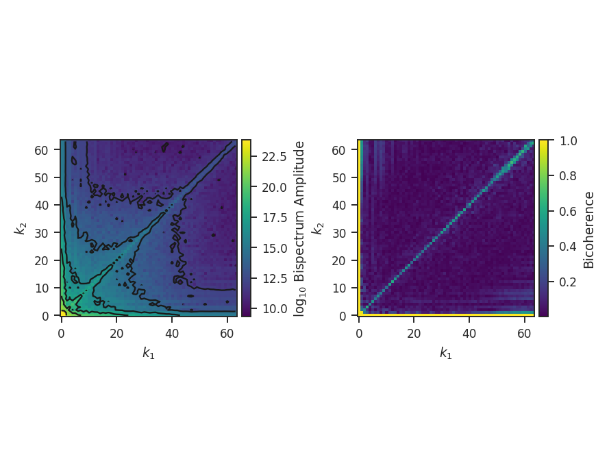
run only performs a single step: compute_bispectrum. For this, there are two optional inputs that may be set:
>>> bispec.run(nsamples=10000, mean_subtract=True, seed=4242424) # doctest: +SKIP
seed sets the random seed for the sampling, and mean_subtract removes the mean from the data before computing the bispectrum. This removes the “zero frequency” power defined based on the largest scale in the image that gives the phase coupling along \(k_1 = k_2\) line. Removing the mean highlights the non-linear mode interactions.
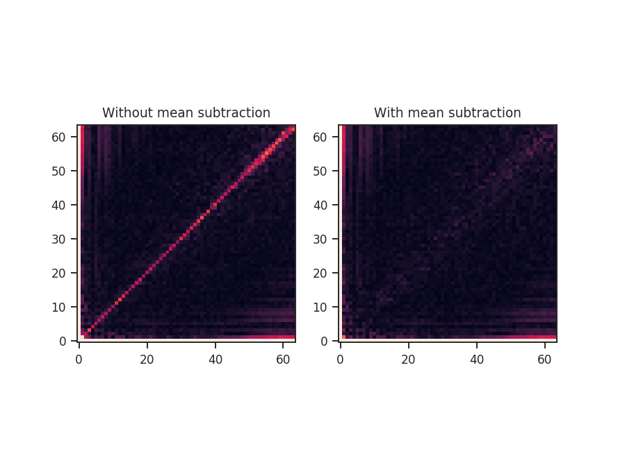
The figure shows the effect on the bicoherence from subtracting the mean. The colorbar is limited between 0 and 1, with black representing 1.
Both radial and azimuthal slices can be extracted from the bispectrum to examine how its properties vary with angle and radius. Using the non-mean subtracted example, radial slices can be returned with:
>>> rad_slices = bispec.radial_slices([30, 45, 60] * u.deg, 20 * u.deg, value='bispectrum_logamp')  # doctest: +SKIP
>>> plt.errorbar(rad_slices[30][0], rad_slices[30][1], yerror=rad_slices[30][2], label='30')  # doctest: +SKIP
>>> plt.errorbar(rad_slices[45][0], rad_slices[45][1], yerror=rad_slices[45][2], label='45')  # doctest: +SKIP
>>> plt.errorbar(rad_slices[60][0], rad_slices[60][1], yerror=rad_slices[60][2], label='60')  # doctest: +SKIP
>>> plt.legend()  # doctest: +SKIP
>>> plt.xlabel("Radius")  # doctest: +SKIP
>>> plt.ylabel("log Bispectrum")  # doctest: +SKIP
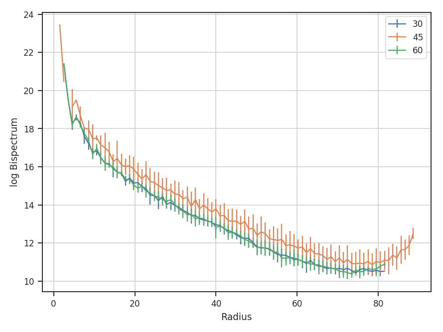
Three slices are returned, centered at 30, 45, and 60 degrees. The width of each slice is 20 degrees. rad_slices is a dictionary whose keys are the (rounded to the nearest integer) center angles given. Each entry in the dictionary has the bin centers ([0]), values ([1]), and standard deviations ([2]). The center angles and slice width can be given in any angular unit. By default, the averaging is over the bispectrum amplitudes. By passing value='bispectrum_logamp', the log of the amplitudes are instead averaged over. The bicoherence array can also be averaged over with value='bicoherence'. The size of the bins can also be changed by passing bin_width to radial_slices; the default is 1.
The azimuthal slices are similarly calculated:
>>> azim_slices = tester.azimuthal_slice([8, 16, 50], 10, value='bispectrum_logamp', bin_width=5 * u.deg)  # doctest: +SKIP
>>> plt.errorbar(azim_slices[8][0], azim_slices[8][1], yerror=azim_slices[8][2], label='8')  # doctest: +SKIP
>>> plt.errorbar(azim_slices[16][0], azim_slices[16][1], yerror=azim_slices[16][2], label='16')  # doctest: +SKIP
>>> plt.errorbar(azim_slices[50][0], azim_slices[50][1], yerror=azim_slices[50][2], label='50')  # doctest: +SKIP
>>> plt.legend()  # doctest: +SKIP
>>> plt.xlabel("Theta (rad)")  # doctest: +SKIP
>>> plt.ylabel("log Bispectrum")  # doctest: +SKIP
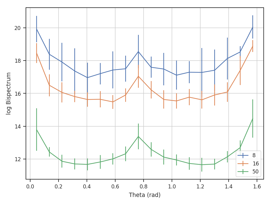
The slices are returned over angles 0 to \(\pi / 2\). With the azimuthal slices, the center radii, in units of the wavevectors, are given and a radial width (10) is specified for all. If different widths are needed, multiple values for the width can be given, though the length must match the length of the center radii.
Delta-Variance
Overview
The \(\Delta\)-variance technique was introduced by Stutzki et al. 1998 as a generalization of Allan-variance, a technique used to study the drift in instrumentation. They found that molecular cloud structures are well characterized by fractional Brownian motion structure, which results from a power-law power spectrum with a random phase distribution. The technique was extended by Bensch et al. 2001. to account for the effects of beam smoothing and edge effects on a discretely sampled grid. With this approach, they identified a functional form to recover the index of the near power-law relation. The technique was extended again by Ossenkopf at al. 2008a, where the computation using filters of different scales was moved into the Fourier domain, allowing for a significant improvement in speed. The following description uses the Fourier-domain formulation.
Delta-variance measures the amount of structure on a given range of scales. Each delta-variance point is calculated by filtering an image with an azimuthally symmetric kernel - a French hat or Mexican hat (Ricker) kernels - and computing the variance of the filtered map. Due to the effects of a finite grid that typically does not have periodic boundaries and the effects of noise, Ossenkopf at al. 2008a proposed a convolution based method that splits the kernel into its central peak and outer annulus, convolves the separate regions, and subtracts the annulus-convolved map from the peak-convolved map. The Mexican-hat kernel separation can be defined using two Gaussian functions. A weight map was also introduced to minimize noise effects where there is low S/N regions in the data. Altogether, this is expressed as:
where \(r\) is the kernel size, \(G\) is the convolved image map, and \(W\) is the convolved weight map. The delta-variance is then,
where \(W_{\rm tot}(r) = W_{\rm core}(r)\,W_{\rm ann}(r)\).
Since the kernel is separated into two components, the ratio between their widths can be set independently. Ossenkopf at al. 2008a find an optimal ratio of 1.5 for the Mexican-hat kernel, which is the element used in TurbuStat.
Performing this operation yields a power-law-like relation between the scales \(r\) and the delta-variance. This power-law relation measured in the real-domain is analogous to the two-point structure function (e.g., Miesch & Bally 1994). Its use of the convolution kernel, as well as handling for map edges, makes it faster to compute and more robust to oddly-shaped regions of signal.
This technique shares many similarities to the Wavelet transform.
Using
The data in this tutorial are available here.
We need to import the DeltaVariance code, along with a few other common packages:
>>> from turbustat.statistics import DeltaVariance
>>> from astropy.io import fits
Then, we load in the data and the associated error array:
>>> moment0 = fits.open("Design4_flatrho_0021_00_radmc_moment0.fits")[0]  # doctest: +SKIP
>>> moment0_err = fits.open("Design4_flatrho_0021_00_radmc_moment0.fits")[1]  # doctest: +SKIP
Next, we initialize the DeltaVariance class:
>>> delvar = DeltaVariance(moment0, weights=moment0_err, distance=250 * u.pc) # doctest: +SKIP
The weight array is optional but is recommended to down-weight noisy data (particularly near the map edge). Note that this is not the exact form of the weight array used by Ossenkopf at al. 2008b; they use the square root of the number of elements along the line of sight used to create the integrated intensity map. This doesn’t take into account the varying S/N of each element used, however. In the case with the simulated data, the two are nearly identical, since the noise value associated with each element is constant. If no weights are given, a uniform array of ones is used.
To compute the delta-variance curve, the image is convolved with a set of kernels. The width of each kernel is referred to as the “lag.” By default, 25 lag values will be used, logarithmically spaced between 3 pixels to half of the minimum axis size. Alternative lags can be specified by setting the lags keyword. If a ndarray is passed, it is assumed to be in pixel units. Lags can also be given in angular units using astropy.units.Quantity objects. The diameter between the inner and outer convolution kernels is set by diam_ratio. By default, this is set to 1.5 (Ossenkopf at al. 2008a).
The entire process is performed through run:
>>> delvar.run(verbose=True, xunit=u.pix)  # doctest: +SKIP
                            WLS Regression Results
==============================================================================
Dep. Variable:                      y   R-squared:                       0.946
Model:                            WLS   Adj. R-squared:                  0.943
Method:                 Least Squares   F-statistic:                     400.2
Date:                Wed, 18 Oct 2017   Prob (F-statistic):           4.80e-16
Time:                        18:38:51   Log-Likelihood:                 13.625
No. Observations:                  25   AIC:                            -23.25
Df Residuals:                      23   BIC:                            -20.81
Df Model:                           1
Covariance Type:            nonrobust
==============================================================================
                 coef    std err          t      P>|t|      [0.025      0.975]
------------------------------------------------------------------------------
const          1.6826      0.036     46.701      0.000       1.608       1.757
x1             1.2654      0.063     20.006      0.000       1.135       1.396
==============================================================================
Omnibus:                        0.195   Durbin-Watson:                   0.506
Prob(Omnibus):                  0.907   Jarque-Bera (JB):                0.403
Skew:                          -0.047   Prob(JB):                        0.818
Kurtosis:                       2.385   Cond. No.                         10.6
==============================================================================
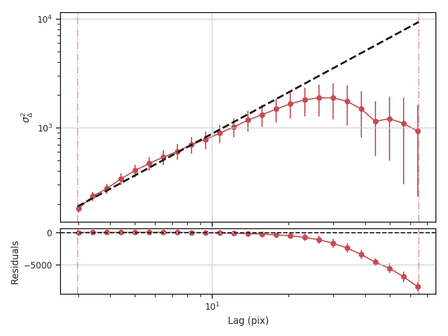
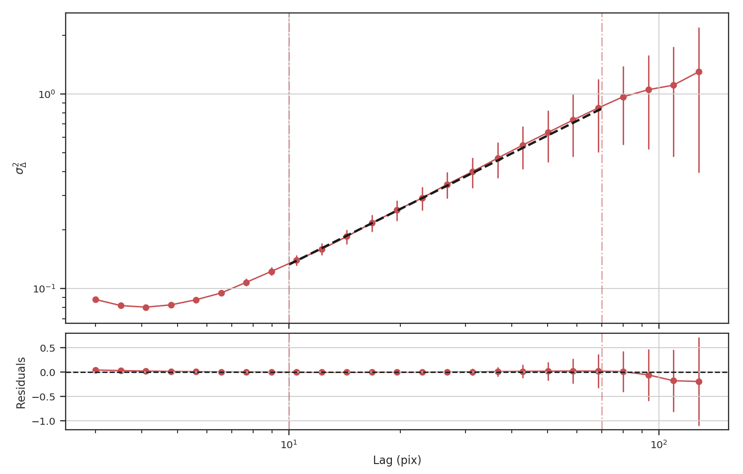
xunit is the unit the lags will be converted to in the plot. The plot includes a linear fit to the Delta-variance curve, however there is a significant deviation from a single power-law on large scales. We can restrict the fitting to reflect this:
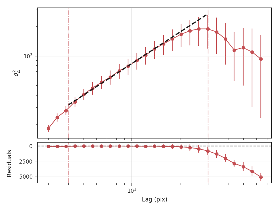
>>> delvar.run(verbose=True, xunit=u.pix, xlow=4 * u.pix, xhigh=30 * u.pix)  # doctest: +SKIP
                            WLS Regression Results
==============================================================================
Dep. Variable:                      y   R-squared:                       0.994
Model:                            WLS   Adj. R-squared:                  0.993
Method:                 Least Squares   F-statistic:                     2167.
Date:                Wed, 18 Oct 2017   Prob (F-statistic):           9.44e-17
Time:                        18:38:52   Log-Likelihood:                 38.238
No. Observations:                  16   AIC:                            -72.48
Df Residuals:                      14   BIC:                            -70.93
Df Model:                           1
Covariance Type:            nonrobust
==============================================================================
                 coef    std err          t      P>|t|      [0.025      0.975]
------------------------------------------------------------------------------
const          1.8620      0.017    106.799      0.000       1.825       1.899
x1             1.0630      0.023     46.549      0.000       1.014       1.112
==============================================================================
Omnibus:                        0.142   Durbin-Watson:                   0.746
Prob(Omnibus):                  0.931   Jarque-Bera (JB):                0.271
Skew:                          -0.182   Prob(JB):                        0.873
Kurtosis:                       2.475   Cond. No.                         11.4
==============================================================================
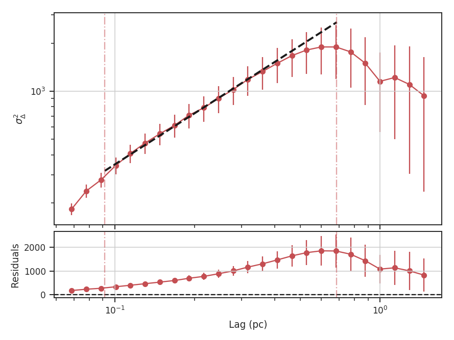
xlow, xhigh, and xunit can also be passed any angular unit, and since a distance was given, physical units can also be passed. For example, using the previous example:
>>> delvar.run(verbose=True, xunit=u.pc, xlow=4 * u.pix, xhigh=30 * u.pix)  # doctest: +SKIP
                            WLS Regression Results
==============================================================================
Dep. Variable:                      y   R-squared:                       0.994
Model:                            WLS   Adj. R-squared:                  0.993
Method:                 Least Squares   F-statistic:                     2167.
Date:                Wed, 18 Oct 2017   Prob (F-statistic):           9.44e-17
Time:                        18:38:52   Log-Likelihood:                 38.238
No. Observations:                  16   AIC:                            -72.48
Df Residuals:                      14   BIC:                            -70.93
Df Model:                           1
Covariance Type:            nonrobust
==============================================================================
                 coef    std err          t      P>|t|      [0.025      0.975]
------------------------------------------------------------------------------
const          1.8620      0.017    106.799      0.000       1.825       1.899
x1             1.0630      0.023     46.549      0.000       1.014       1.112
==============================================================================
Omnibus:                        0.142   Durbin-Watson:                   0.746
Prob(Omnibus):                  0.931   Jarque-Bera (JB):                0.271
Skew:                          -0.182   Prob(JB):                        0.873
Kurtosis:                       2.475   Cond. No.                         11.4
==============================================================================
Since the Delta-variance is based on a series of convolutions, there is a choice for how the boundaries should be treated. This is set by the boundary keyword in run. By default, boundary='wrap' as is appropriate for simulated data in a periodic box. If the data is not periodic in the spatial dimensions, boundary='fill' should be used. This mode pads the edges of the data based on the size of the convolution kernel used.
When an image contains NaNs, there are two important parameters for the convolution: preserve_nan and nan_treatment. Setting preserve_nan=True will set pixels that were originally a NaN to a NaN in the convolved image. This is useful for when the image has a border of NaNs. When the edges are not handled correctly, the delta-variance curve will have large spikes at small lag values.
If an image has missing values within the image, setting nan_treatment='interpolate' will interpolate over the missing regions, providing a smoothed version of the convolved image. However, interpolation may perform poorly when the image has a border of NaNs. In this case, nan_treatment='fill' will fill NaN values with a constant value (the default is \(0.0\)). Since the edge effects may be extreme with interpolation, the default setting is nan_treatment='fill'.
If an image has both missing regions and a border of NaNs, manual treatment may be necessary to convert the edges to NaNs while correctly handling the interpolating regions in the interior. See the convolution page on astropy for more information.
Similar to the fitting for other statistics, the Delta-variance curve can be fit with a segmented linear model:
>>> delvar.run(verbose=True, xunit=u.pc, xlow=4 * u.pix, xhigh=40 * u.pix, brk=8 * u.pix)  # doctest: +SKIP
                            WLS Regression Results
==============================================================================
Dep. Variable:                      y   R-squared:                       0.996
Model:                            WLS   Adj. R-squared:                  0.995
Method:                 Least Squares   F-statistic:                     1168.
Date:                Thu, 19 Oct 2017   Prob (F-statistic):           4.97e-17
Time:                        15:36:23   Log-Likelihood:                 45.438
No. Observations:                  18   AIC:                            -82.88
Df Residuals:                      14   BIC:                            -79.31
Df Model:                           3
Covariance Type:            nonrobust
==============================================================================
                 coef    std err          t      P>|t|      [0.025      0.975]
------------------------------------------------------------------------------
const          1.8454      0.015    121.610      0.000       1.813       1.878
x1             1.0860      0.020     54.133      0.000       1.043       1.129
x2            -1.1586      0.253     -4.585      0.000      -1.701      -0.617
x3            -0.0064      0.042     -0.153      0.881      -0.096       0.083
==============================================================================
Omnibus:                        0.130   Durbin-Watson:                   1.082
Prob(Omnibus):                  0.937   Jarque-Bera (JB):                0.037
Skew:                           0.009   Prob(JB):                        0.982
Kurtosis:                       2.778   Cond. No.                         127.
==============================================================================
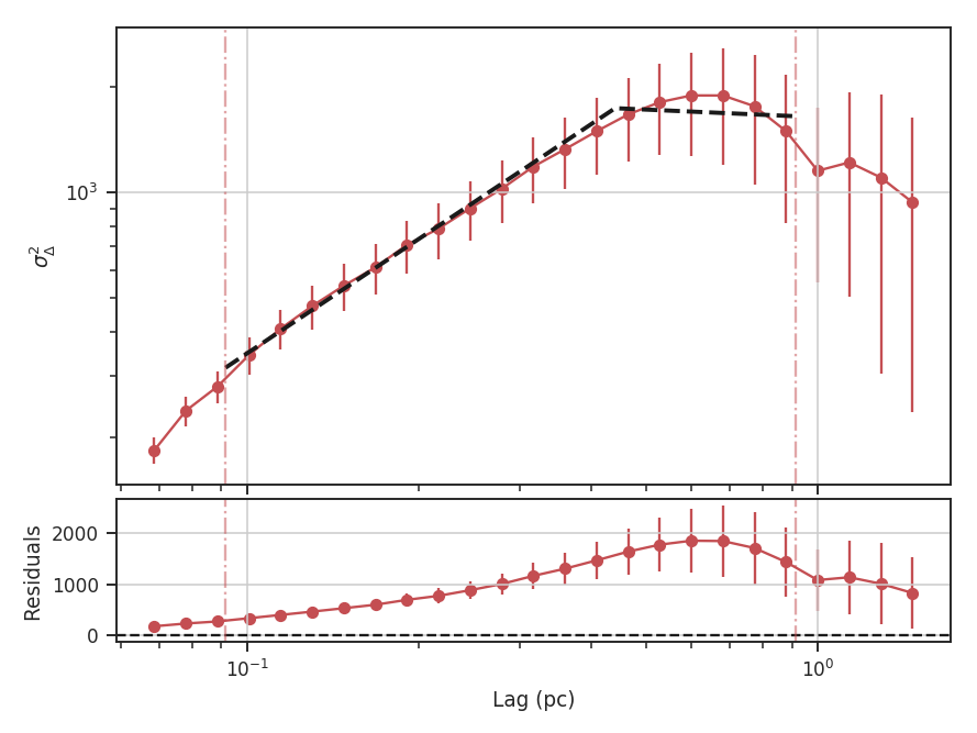
The range here was chosen to force the model to fit a break near the turn-over, and the result is not great. This is not a realistic example; it is included only to highlight how the segmented model is enabled.
There will now be two slopes and a break point returned:
>>> delvar.slope  # doctest: +SKIP
array([ 1.08598566, -0.07259903])
>>> delvar.brk  # doctest: +SKIP
<Quantity 19.413294229328802 pix>
Warning
The turn-over at large scales (usually larger than half the image size) tends to be dominated by the kernel shape rather than the data. On scales smaller than the beam size, the curve will tend to steepen. This is due to the enhanced correlations from over-sampling the beam, which is standard for radio and submillimetre observational data. See Bensch et al. 2001. for a discussion of how the beam affects the delta-variance curves.
Volker Ossenkopf-Okada’s IDL Delta-Variance codes is available here.
Dendrograms
Overview
In general, dendrograms provide a hierarchical description of datasets, which may be used to identify clusters of similar objects or variables. This is known as hierarchical clustering. In the case of position-position-velocity (PPV) cubes, a dendrogram is a hierarchical decomposition of the emission in the cube. This decomposition was introduced by Rosolowsky et al. 2008 and Goodman et al. 2009 to calculate the multiscale properties of molecular gas in nearby clouds. The tree structure is comprised of branches and leaves. Branches are the connections, while leaves are the tips of the branches.
Burkhart et al. 2013 introduced two statistics for comparing the dendrograms of two cubes: the relationship between the number of leaves and branches in the tree versus the minimum branch length, and a histogram comparison of the peak intensity in a branch or leaf. The former statistic shows a power-law like turn-off with increasing branch length.
Using
The data in this tutorial are available here.
Requires the optional astrodendro package to be installed. See the documentation
Importing the dendrograms code, along with a few other common packages:
>>> from turbustat.statistics import Dendrogram_Stats
>>> from astropy.io import fits
>>> import astropy.units as u
>>> from astrodendro import Dendrogram
>>> import matplotlib.pyplot as plt
>>> import numpy as np
And we load in the data:
>>> cube = fits.open("Design4_flatrho_0021_00_radmc.fits")[0]
Before running the statistics side, we can first compute the dendrogram itself to see what we’re dealing with:
>>> d = Dendrogram.compute(cube.data, min_value=0.005, min_delta=0.1, min_npix=50, verbose=True)
>>> ax = plt.subplot(111)
>>> d.plotter().plot_tree(ax)
>>> plt.ylabel("Intensity (K)")
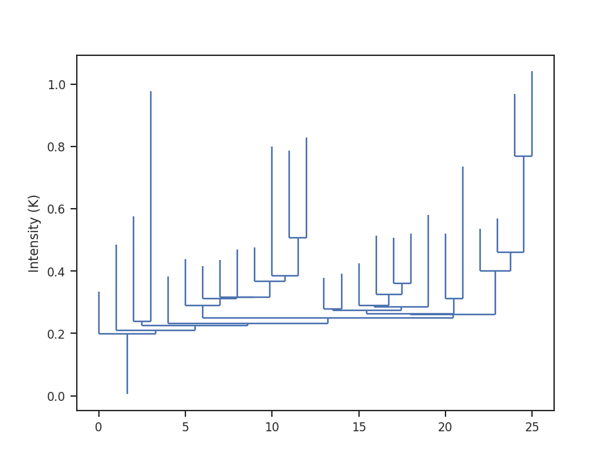
We see a number of leaves of varying height throughout the tree. Their minimum height is set by min_delta. As we increase this value, the tree becomes pruned: more and more structure will be merged, leaving only the brightest regions on the tree.
While this tutorial uses a PPV cube, a 2D image may also be used! The same tutorial code can be used for both, with changes needed for the choice of min_delta.
The statistics are computed through Dendrogram_Stats:
>>> dend_stat = Dendrogram_Stats(cube,
...                              min_deltas=np.logspace(-2, 0, 50),
...                              dendro_params={"min_value": 0.005, "min_npix": 50})
There are two parameters that will change depending on the given data set: (1) min_deltas sets the minimum branch heights, which are completely dependent on the range of values within the data data, and (2) dendro_params, which is a dictionary setting other dendrogram parameters such as the minimum number of pixels a region must have (min_npix) and the minimum values of the data to consider (min_value). The settings given above are specific for these data and will need to be changed when using other data sets.
To run the statistics, we use run:
>>> dend_stat.run(verbose=True)
                            OLS Regression Results
==============================================================================
Dep. Variable:                      y   R-squared:                       0.962
Model:                            OLS   Adj. R-squared:                  0.960
Method:                 Least Squares   F-statistic:                     825.6
Date:                Mon, 03 Jul 2017   Prob (F-statistic):           6.25e-25
Time:                        15:04:02   Log-Likelihood:                 34.027
No. Observations:                  35   AIC:                            -64.05
Df Residuals:                      33   BIC:                            -60.94
Df Model:                           1
Covariance Type:            nonrobust
==============================================================================
                 coef    std err          t      P>|t|      [0.025      0.975]
------------------------------------------------------------------------------
const          0.4835      0.037     13.152      0.000       0.409       0.558
x1            -1.1105      0.039    -28.733      0.000      -1.189      -1.032
==============================================================================
Omnibus:                        4.273   Durbin-Watson:                   0.287
Prob(Omnibus):                  0.118   Jarque-Bera (JB):                3.794
Skew:                          -0.800   Prob(JB):                        0.150
Kurtosis:                       2.800   Cond. No.                         4.39
==============================================================================
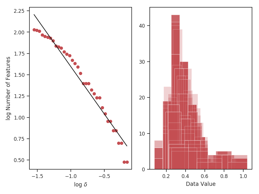
On the left is the relationship between the value of min_delta and the number of features in the tree. On the right is a stack of histograms, showing the distribution of peak intensities for all values of min_delta. The results of the linear fit are also printed, where x1 is the slope of the power-law tail.
When using simulated data from a periodic box, the boundaries need to be handled across the edges. Setting periodic_bounds=True will treat the spatial dimensions as periodic. The simulated data shown here should have periodic_bounds enabled:
>>> dend_stat.run(verbose=True, periodic_bounds=True)
                            OLS Regression Results
==============================================================================
Dep. Variable:                      y   R-squared:                       0.962
Model:                            OLS   Adj. R-squared:                  0.961
Method:                 Least Squares   F-statistic:                     808.6
Date:                Thu, 06 Jul 2017   Prob (F-statistic):           2.77e-24
Time:                        13:30:48   Log-Likelihood:                 33.415
No. Observations:                  34   AIC:                            -62.83
Df Residuals:                      32   BIC:                            -59.78
Df Model:                           1
Covariance Type:            nonrobust
==============================================================================
                 coef    std err          t      P>|t|      [0.025      0.975]
------------------------------------------------------------------------------
const          0.3758      0.039      9.744      0.000       0.297       0.454
x1            -1.1369      0.040    -28.437      0.000      -1.218      -1.055
==============================================================================
Omnibus:                        4.386   Durbin-Watson:                   0.267
Prob(Omnibus):                  0.112   Jarque-Bera (JB):                4.055
Skew:                          -0.823   Prob(JB):                        0.132
Kurtosis:                       2.611   Cond. No.                         4.60
==============================================================================
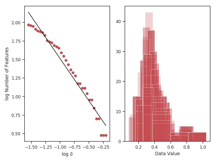
The results have slightly changed. The left panel shows fewer features at nearly every value of \(\delta\) as regions along the edges are connected across the boundaries.
Creating the initial dendrogram is the most time-consuming step. To check the progress of building the dendrogram, dendro_verbose=True can be set in the previous call to give a progress bar and time-to-completion estimate.
Computing dendrograms can be time-consuming when working with large datasets. We can avoid recomputing a dendrogram by loading from an HDF5 file:
>>> dend_stat = Dendrogram_Stats.load_dendrogram("design4_dendrogram.hdf5",
...                                              min_deltas=np.logspace(-2, 0, 50))
Saving the dendrogram structure is explained in the astrodendro documentation. The saved dendrogram must have min_delta set to the minimum of the given min_deltas. Otherwise pruning is ineffective.
If the dendrogram is stored in a variable (say you have just run it in the same terminal), you may pass the computed dendrogram into run:
>>> d = Dendrogram.compute(cube, min_value=0.005, min_delta=0.01, min_npix=50, verbose=True)
>>> dend_stat = Dendrogram_Stats(cube, min_deltas=np.logspace(-2, 0, 50))
>>> dend_stat.run(verbose=True, dendro_obj=d)
Once the statistics have been run, the results can be saved as a pickle file:
>>> dend_stat.save_results(output_name="Design4_Dendrogram_Stats.pkl", keep_data=False)
keep_data=False will avoid saving the entire cube and is the default setting.
Saving can also be enabled with run:
>>> dend_stat.run(save_results=True, output_name="Design4_Dendrogram_Stats.pkl")
The results may then be reloaded:
>>> dend_stat = Dendrogram_Stats.load_results("Design4_Dendrogram_Stats.pkl")
Note that the dendrogram and data are NOT saved, and only the statistic outputs will be accessible.
Genus
Overview
Genus statistics provide a measure of a region’s topology. At a given value in the data, the Genus value is the number of discrete regions above the value minus the number of regions below it. When this process is repeated over a range of values, a Genus curve can be constructed. The technique has previously been used to study CMB deviations from a Gaussian distribution.
If a region has a negative Genus statistics, it is dominated by holes in the emission (“swiss cheese” morphology). A positive Genus value implies a “meatball” morphology, where the emission is localized into clumps. The Genus curve of a Gaussian field is shown below. Note that at the mean value (0.0), the Genus value is zero: at the mean intensity, there is no preference to either morphological type.
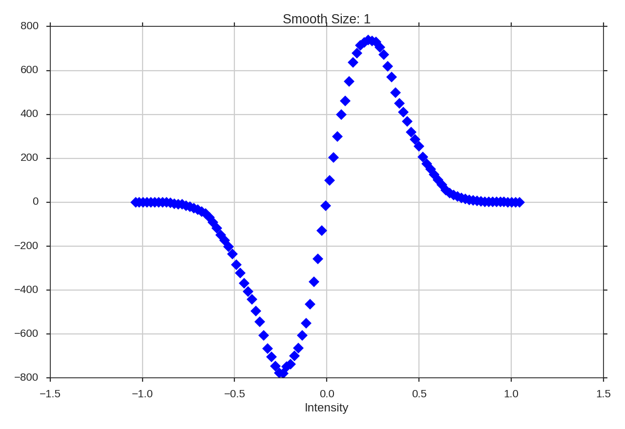
Kowal et al. 2007 constructed Genus curves for a set of simulations to investigate the effect of changing the Mach number and the Alfvenic Mach number. The isocontours were taken for a range of density values in the full position-position-position space. Applications to observations includes Chepurnov et al. 2008 and Burkhart et al. 2012.
Using
The data in this tutorial are available here.
We need to import the Genus code, along with a few other common packages:
>>> from turbustat.statistics import Genus
>>> from astropy.io import fits
>>> import astropy.units as u
>>> import numpy as np
And we load in the data:
>>> moment0 = fits.open("Design4_flatrho_0021_00_radmc_moment0.fits")[0] # doctest: +SKIP
The FITS HDU is passed to initialize Genus:
>>> genus = Genus(moment0, lowdens_percent=15, highdens_percent=85, numpts=100,
...               smoothing_radii=np.linspace(1, moment0.shape[0] / 10., 5))  # doctest: +SKIP
lowdens_percent and highdens_percent set the upper and lower percentiles in the data to measure the Genus value at. When using observational data, lowdens_percent should be set above the noise level. Alternatively, specific values for the low and high cut-offs can be passed using min_value and max_value, respectively. The min_value and max_value settings are overridden when lowdens_percent > min_value or highdens_percent < max_value.
The numpts parameter sets how many Genus values to compute between the given percentiles. Finally, smoothing_radii allows for the data to be smoothed, minimizing the influence of noise on the Genus curve at the expense of resolution. The values given are used as the radii of a Gaussian smoothing kernel. The values given above (np.linspace(1, moment0.shape[0] / 10., 5)) are used by default when no values are given.
Computing the curves is accomplished using run:
>>> genus.run(verbose=True, min_size=4) # doctest: +SKIP
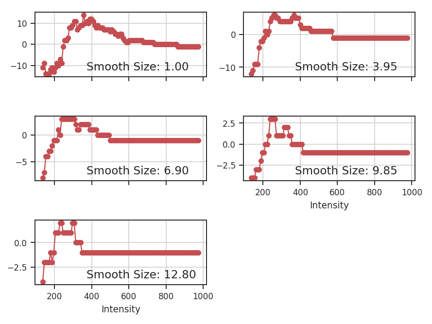
If min_value and max_value are set instead:
>>> genus = Genus(moment0, min_value=137, max_value=353, numpts=100)  # doctest: +SKIP
>>> genus.run(verbose=True, min_size=4)  # doctest: +SKIP

I have set min_value and max_value to the same percentiles used above and so we get the same result.
The basic sinusoid seen in the Genus curve of the Gaussian field is still evident. As we smooth the data on larger scales, the topological information is lost, and the curve becomes degraded. To avoid spurious noise features, the minimum area a region must have to be considered is set by min_size. This is simulated data, so a small value has been chosen.
Often the smallest size that can be “trusted” in a radio image is the beam area. In this example, a FITS HDU was passed, including an associated header. If the beam information is contained in the header, the size threshold can be set to the beam area using use_beam=True:
>>> moment0.header["BMAJ"] = 2e-5  # deg.   # doctest: +SKIP
>>> genus = Genus(moment0, lowdens_percent=15, highdens_percent=85,
...               smoothing_radii=[1] * u.pix)  # doctest: +SKIP
>>> genus.run(verbose=True, use_beam=True)  # doctest: +SKIP
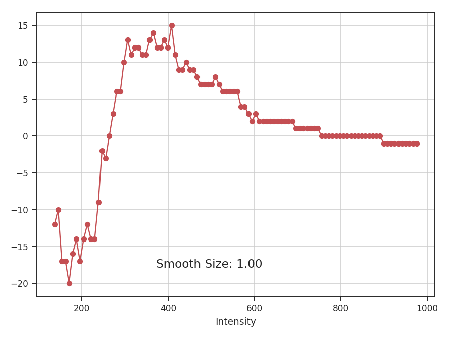
The curve has far less detail than in the earlier example because of the new requirement for large, connected regions. Note that the FITS keywords “BMIN” and “BPA” are also read and used when available. More options for reading beam information are available when the optional package radio_beam is installed. If the beam information is not contained in the header, or you wish to use any other minimum area, the size can be passed using min_size. To get the same result as the last example:
>>> genus.run(verbose=True, use_beam=True, min_size=2e-5**2 * np.pi * u.deg**2) # doctest: +SKIP
If a distance is given to Genus, areas and smoothing radii can be passed in physical units:
>>> genus = Genus(moment0, lowdens_percent=15, highdens_percent=85,
...               smoothing_radii=u.Quantity([0.04 * u.pc]), distance=500 * u.pc)  # doctest: +SKIP
>>> genus.run(verbose=True, min_size=40 * u.AU**2)  # doctest: +SKIP
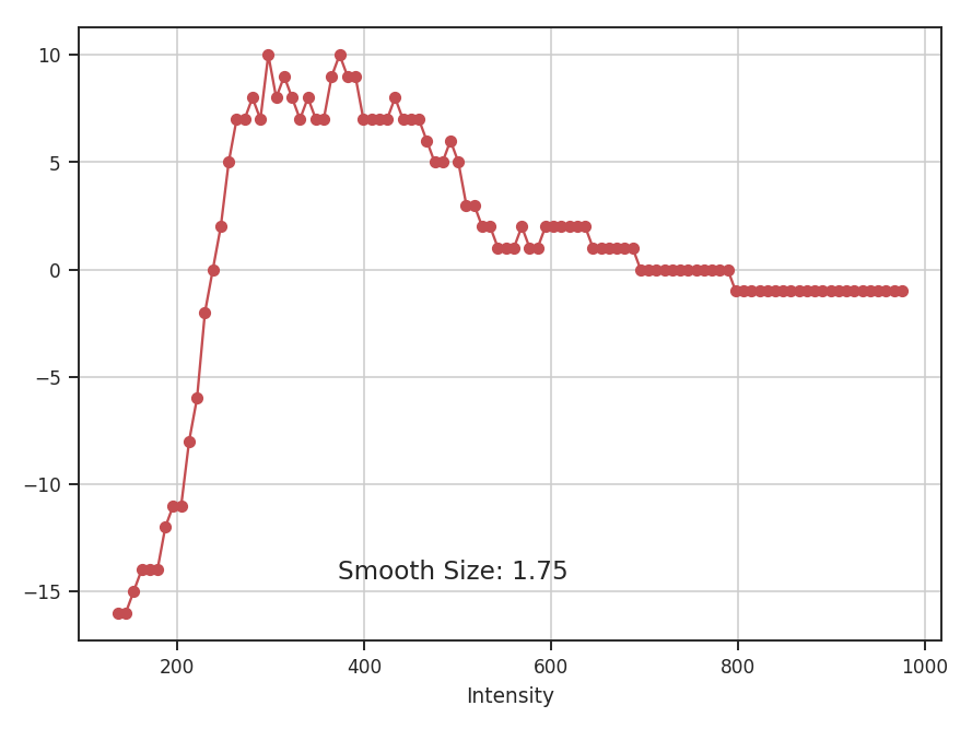
Note that the smooth size shown in the plots is always the smoothing radius in pixels.
Modified Velocity Centroids
Overview
Centroid statistics have been used to study molecular clouds for decades. For example, Miesch & Bally 1994 created structure functions of the centroid surfaces from CO data in a number of nearby clouds. The slope of the structure function is one way to measure the size-line width relation of a region. The normalized centroids take the form
where \(I(x, v)\) is a PPV cube with \(x\) representing the spatial coordinate, \(v\) the velocity coordinate, and \(M_0\) the integrated intensity (moment zero). On small scales, however, the contribution from density fluctuations can dominate, and the first moment is contaminated on these small scales. These centroids make sense intuitively, however, since this is simply the mean weighted by the intensity. Lazarian & Esquivel 2003 proposed Modified Velocity Centroids (MVC) as a technique to remove the small scale density contamination. This involves an unnormalized centroid
The structure function of the modified velocity centroid is then the squared difference of the unnormalized centroid with the squared difference of \(M_0\) times the velocity dispersion (\(<v^2>\)) subtracted to remove the density contribution. This is both easier to express and compute in the Fourier domain, which yields a two-dimensional power spectrum:
where \(\mathcal{M}_i\) denotes the Fourier transform of the ith moment. MVC is also explored in Esquivel & Lazarian 2005.
Using
The data in this tutorial are available here.
We need to import the MVC code, along with a few other common packages:
>>> from turbustat.statistics import MVC
>>> from astropy.io import fits
Most statistics in TurbuStat require only a single data input. MVC requires 3, as you can see in the last equation. The zeroth (integrated intensity), first (centroid), and second (velocity dispersion) moments of the data cube are needed:
>>> moment0 = fits.open("Design4_flatrho_0021_00_radmc_moment0.fits")[0]  # doctest: +SKIP
>>> moment1 = fits.open("Design4_flatrho_0021_00_radmc_centroid.fits")[0]  # doctest: +SKIP
>>> lwidth = fits.open("Design4_flatrho_0021_00_radmc_linewidth.fits")[0]  # doctest: +SKIP
The unnormalized centroid can be recovered by multiplying the normal centroid value by the zeroth moment. The line width array here is the square root of the velocity dispersion. These three arrays must be passed to MVC:
>>> mvc = MVC(moment1, moment0, lwidth) # doctest: +SKIP
The header is read in from moment1 to convert into angular scales. Alternatively, a different header can be given with the header keyword.
Calculating the power spectrum, radially averaging, and fitting a power-law are accomplished through the run command:
>>> mvc.run(verbose=True, xunit=u.pix**-1)  # doctest: +SKIP
                            OLS Regression Results
==============================================================================
Dep. Variable:                      y   R-squared:                       0.941
Model:                            OLS   Adj. R-squared:                  0.941
Method:                 Least Squares   F-statistic:                     1425.
Date:                Mon, 10 Jul 2017   Prob (F-statistic):           1.46e-56
Time:                        16:34:01   Log-Likelihood:                -52.840
No. Observations:                  91   AIC:                             109.7
Df Residuals:                      89   BIC:                             114.7
Df Model:                           1
Covariance Type:            nonrobust
==============================================================================
                 coef    std err          t      P>|t|      [0.025      0.975]
------------------------------------------------------------------------------
const         14.0317      0.103    136.541      0.000      13.827      14.236
x1            -5.0142      0.133    -37.755      0.000      -5.278      -4.750
==============================================================================
Omnibus:                        3.535   Durbin-Watson:                   0.129
Prob(Omnibus):                  0.171   Jarque-Bera (JB):                3.484
Skew:                          -0.468   Prob(JB):                        0.175
Kurtosis:                       2.796   Cond. No.                         4.40
==============================================================================
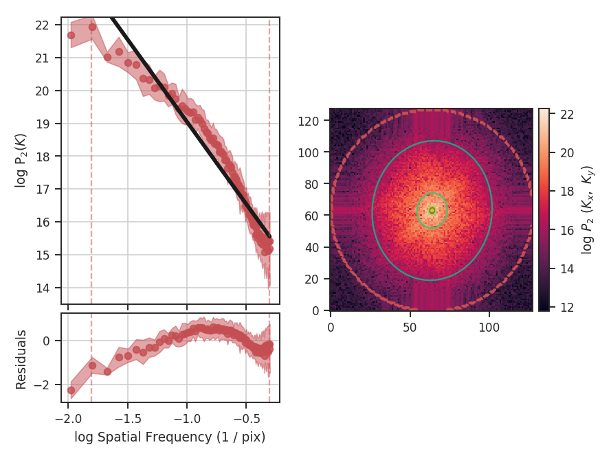
The code returns a summary of the one-dimensional fit and a figure showing the one-dimensional spectrum and model on the left, and the two-dimensional power-spectrum on the right. If fit_2D=True is set in run (the default setting), the contours on the two-dimensional power-spectrum are the fit using an elliptical power-law model. We will discuss the models in more detail below. The dashed red lines (or contours) on both plots are the limits of the data used in the fits. See the PowerSpectrum tutorial for a discussion of the two-dimensional fitting.
The fit here is not very good since the spectrum deviates from a single power-law on small scales. In this case, the deviation is caused by the limited inertial range in the simulation from which this spectral-line data cube was created. We can specify low_cut and high_cut in frequency units to limit the fitting to the inertial range:
>>> mvc.run(verbose=True, xunit=u.pix**-1, low_cut=0.02 / u.pix, high_cut=0.1 / u.pix)  # doctest: +SKIP
                            OLS Regression Results
==============================================================================
Dep. Variable:                      y   R-squared:                       0.952
Model:                            OLS   Adj. R-squared:                  0.948
Method:                 Least Squares   F-statistic:                     255.9
Date:                Mon, 10 Jul 2017   Prob (F-statistic):           6.22e-10
Time:                        16:34:01   Log-Likelihood:                 10.465
No. Observations:                  15   AIC:                            -16.93
Df Residuals:                      13   BIC:                            -15.51
Df Model:                           1
Covariance Type:            nonrobust
==============================================================================
                 coef    std err          t      P>|t|      [0.025      0.975]
------------------------------------------------------------------------------
const         16.7121      0.220     75.957      0.000      16.237      17.187
x1            -2.7357      0.171    -15.997      0.000      -3.105      -2.366
==============================================================================
Omnibus:                        0.814   Durbin-Watson:                   2.077
Prob(Omnibus):                  0.666   Jarque-Bera (JB):                0.614
Skew:                          -0.445   Prob(JB):                        0.736
Kurtosis:                       2.564   Cond. No.                         13.5
==============================================================================
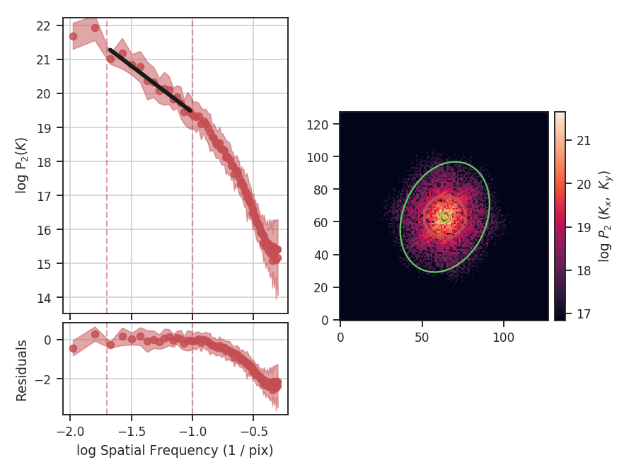
Note the drastic change in the slope! Specifying the correct fit region for the data you are using is critical for interpreting the results of the method. This example has used the default ordinary least-squares fitting. A weighted least-squares can be enabled with weighted_fit=True (this cannot be used for the segmented model described below).
Breaks in the power-law behaviour in observations (and higher-resolution simulations) can result from differences in the physical processes dominating at those scales. To capture this behaviour, MVC can be passed a break point to enable fitting with a segmented linear model (Lm_Seg). Note that the 2D fitting is disabled for this section as it does not handle fitting break points. From the above plot, we can estimate the break point to be near 0.1 / u.pix:
>>> mvc.run(verbose=True, xunit=u.pix**-1, low_cut=0.02 / u.pix,
...         high_cut=0.4 / u.pix,
...         fit_kwargs=dict(brk=0.1 / u.pix), fit_2D=False)  # doctest: +SKIP
                            OLS Regression Results
==============================================================================
Dep. Variable:                      y   R-squared:                       0.994
Model:                            OLS   Adj. R-squared:                  0.994
Method:                 Least Squares   F-statistic:                     4023.
Date:                Mon, 10 Jul 2017   Prob (F-statistic):           1.50e-75
Time:                        16:41:34   Log-Likelihood:                 53.269
No. Observations:                  71   AIC:                            -98.54
Df Residuals:                      67   BIC:                            -89.49
Df Model:                           3
Covariance Type:            nonrobust
==============================================================================
                 coef    std err          t      P>|t|      [0.025      0.975]
------------------------------------------------------------------------------
const         16.1749      0.094    172.949      0.000      15.988      16.362
x1            -3.1436      0.085    -36.870      0.000      -3.314      -2.973
x2            -5.0895      0.205    -24.855      0.000      -5.498      -4.681
x3            -0.0020      0.054     -0.037      0.970      -0.110       0.106
==============================================================================
Omnibus:                        9.161   Durbin-Watson:                   1.074
Prob(Omnibus):                  0.010   Jarque-Bera (JB):                8.815
Skew:                          -0.747   Prob(JB):                       0.0122
Kurtosis:                       3.865   Cond. No.                         21.5
==============================================================================

brk is the initial guess at where the break point is. Here I’ve set it to near the extent of the inertial range of the simulation. log_break should be enabled if the given brk is already the log (base-10) value (since the fitting is done in log-space). The segmented linear model iteratively optimizes the location of the break point, trying to minimize the gap between the different components. This is the x3 parameter above. The slopes of the components are x1 and x2, but the second slope is defined relative to the first slope (i.e., if x2=0, the slopes of the components would be the same). The true slopes can be accessed through mvc.slope and mvc.slope_err. The location of the fitted break point is given by mvc.brk, and its uncertainty mvc.brk_err. If the fit does not find a good break point, it will revert to a linear fit without the break.
Many of the techniques in TurbuStat are derived from two-dimensional power spectra. Because of this, the radial averaging and fitting code for these techniques are contained within a common base class, StatisticBase_PSpec2D. Fitting options may be passed as keyword arguments to run. Alterations to the power-spectrum binning can be passed in compute_radial_pspec, after which the fitting routine (fit_pspec) may be run.
The frequency units of the final plot (xunit) and the units of low_cut and high_cut can be given in angular units, as well as physical units when a distance is given. For example:
>>> mvc = MVC(centroid, moment0, lwidth, distance=250 * u.pc)  # doctest: +SKIP
>>> mvc.run(verbose=True, xunit=u.pc**-1, low_cut=0.02 / u.pix,
...         high_cut=0.1 / u.pix, fit_2D=False)  # doctest: +SKIP
                            OLS Regression Results
==============================================================================
Dep. Variable:                      y   R-squared:                       0.952
Model:                            OLS   Adj. R-squared:                  0.948
Method:                 Least Squares   F-statistic:                     255.9
Date:                Sun, 16 Jul 2017   Prob (F-statistic):           6.22e-10
Time:                        14:18:45   Log-Likelihood:                 10.465
No. Observations:                  15   AIC:                            -16.93
Df Residuals:                      13   BIC:                            -15.51
Df Model:                           1
Covariance Type:            nonrobust
==============================================================================
                 coef    std err          t      P>|t|      [0.025      0.975]
------------------------------------------------------------------------------
const         16.7121      0.220     75.957      0.000      16.237      17.187
x1            -2.7357      0.171    -15.997      0.000      -3.105      -2.366
==============================================================================
Omnibus:                        0.814   Durbin-Watson:                   2.077
Prob(Omnibus):                  0.666   Jarque-Bera (JB):                0.614
Skew:                          -0.445   Prob(JB):                        0.736
Kurtosis:                       2.564   Cond. No.                         13.5
==============================================================================

Alternatively, the fitting limits could be passed in units of u.pc**-1.
Constraints on the azimuthal angles used to compute the one-dimensional power-spectrum can also be given:
>>> mvc = MVC(centroid, moment0, lwidth, distance=250 * u.pc)  # doctest: +SKIP
>>> mvc.run(verbose=True, xunit=u.pc**-1, low_cut=0.02 / u.pix, high_cut=0.1 / u.pix,
...         fit_2D=False,
...         radial_pspec_kwargs={"theta_0": 1.13 * u.rad, "delta_theta": 40 * u.deg})  # doctest: +SKIP
                            OLS Regression Results
==============================================================================
Dep. Variable:                      y   R-squared:                       0.806
Model:                            OLS   Adj. R-squared:                  0.791
Method:                 Least Squares   F-statistic:                     53.85
Date:                Fri, 29 Sep 2017   Prob (F-statistic):           5.68e-06
Time:                        14:51:27   Log-Likelihood:                 1.4445
No. Observations:                  15   AIC:                             1.111
Df Residuals:                      13   BIC:                             2.527
Df Model:                           1
Covariance Type:            nonrobust
==============================================================================
                 coef    std err          t      P>|t|      [0.025      0.975]
------------------------------------------------------------------------------
const         17.3709      0.401     43.271      0.000      16.504      18.238
x1            -2.2897      0.312     -7.338      0.000      -2.964      -1.616
==============================================================================
Omnibus:                        1.198   Durbin-Watson:                   2.743
Prob(Omnibus):                  0.549   Jarque-Bera (JB):                0.809
Skew:                          -0.185   Prob(JB):                        0.667
Kurtosis:                       1.924   Cond. No.                         13.5
==============================================================================
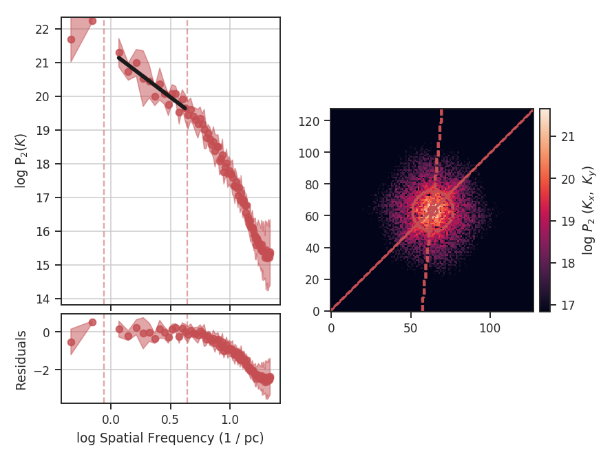
The azimuthal limits now appear as contours on the two-dimensional power-spectrum in the figure. See the PowerSpectrum tutorial for more information on giving azimuthal constraints.
If strong emission continues to the edge of the map (and the map does not have periodic boundaries), ringing in the FFT can introduce a cross pattern in the 2D power-spectrum. This effect and the use of apodizing kernels to taper the data is covered here.
Most observational data will be smoothed over the beam size, which will steepen the power spectrum on small scales. To account for this, the 2D power spectrum can be divided by the beam response. This is demonstrated here for spatial power-spectra.
PCA
Overview
Principal Component Analysis (PCA) is primarily a dimensionality reduction technique. Generally the data are arranged into a set of columns (representing dimensions or variables) and the set of samples is contained within each row. A covariance matrix is then constructed between each pair of columns. Performing an eigenvalue decomposition of this matrix gives an orthogonal basis for the data, the components of which are the principal components (eigenvectors). The associated eigenvalues correspond to the variance in the data described by each principal component.
By ordering the principal components from the largest to smallest eigenvalue, a minimal set of eigenvectors can be found that account for a large portion of the variance within the data. These first N principal components have a (usually) much reduced dimensionality, while still containing the majority of the structure in the data. The PCA Wikipedia page has a much more thorough explanation.
The use of PCA on spectral-line data cubes was introduced by Heyer & Schloerb 1997, and thoroughly extended in a number of other papers (e.g., Brunt & Heyer 2002a, Brunt & Heyer 2002b, Roman-Duval et al. 2011). An analytical derivation is given in Brunt & Heyer 2013. Briefly, they use the PCA decomposition to measure the associated spectral and spatial width scales associated with each principal component. An eigenvalue can be multiplied by each spectral channel to produce an eigenimage. The autocorrelation function of that eigenimage gives an estimate of the spatial scale of that principal component. The autocorrelation of the eigenvector itself gives an associated spectral width. Using the spatial and spectral widths from the first N principal components give an estimate of the size-line width relation.
Using
The data in this tutorial are available here.
We need to import the PCA code, along with a few other common packages:
>>> from turbustat.statistics import PCA
>>> from astropy.io import fits
>>> import astropy.units as u
>>> import matplotlib.pyplot as plt
And we load in the data:
>>> cube = fits.open("Design4_flatrho_0021_00_radmc.fits")[0] # doctest: +SKIP
The PCA class is first initialized, and the distance to the region (if desired) can be given:
>>> pca = PCA(cube, distance=250. * u.pc) # doctest: +SKIP
If the distance is given, you will have the option to convert spatial widths to physical units. Note that we’re using simulated data and the distance of 250 pc has no special meaning in this case. If no distance is provided, conversions to the physical units will return an error.
The simplest way to run the entire process is using the run command:
>>> pca.run(verbose=True, min_eigval=1e-4, spatial_output_unit=u.pc,
...         spectral_output_unit=u.m / u.s, brunt_beamcorrect=False)  # doctest: +SKIP
Proportion of Variance kept: 0.9996934513444623
Index: 0.72 (0.70, 0.73)
Gamma: 0.90 (0.55, 1.26)
Sonic length: 4.419e+00 (3.306e+00, 5.532e+00) pix at 10.0 K

Note that we have specified the output units for the spectral and spatial units. By default, these would be kept in pixel units.
The key properties are shown when verbose=True: a summary of the results with a plot of the covariance matrix (top left), the variance described by the principal components (bottom left) and the size-line width relation (right). The proportion of variance is the variance contained in the N eigenvalues kept. In this case, we consider all eigenvalues with values above 1e-4 to be important. In observational data, min_eigval should be set to the variance of the noise (square of the rms uncertainty). Typically, only the first \(\sim10\) eigenvalues contain signal in observational data.
In the output above index is the slope of the size-line width relation, and gamma is the the slope with a correction factor applied (see gamma). The sonic length is derived from the intercept of the size-line width relation using a default temperature of 10 K (see below on how to change this).
Since these data are simulated, this example does not account for a finite beam size. If it did, however, we would want to deconvolve the spatial widths with the beam. To see this effect, let us assume these data have a 20” circular beam:
>>> pca.run(verbose=True, min_eigval=1e-4, spatial_output_unit=u.pc,
...         spectral_output_unit=u.m / u.s, brunt_beamcorrect=True,
...         beam_fwhm=10 * u.arcsec)  # doctest: +SKIP
Proportion of Variance kept: 0.9996934513444623
Index: 0.71 (0.70, 0.73)
Gamma: 0.89 (0.54, 1.25)
Sonic length: 4.394e+00 (3.284e+00, 5.505e+00) pix at 10.0 K
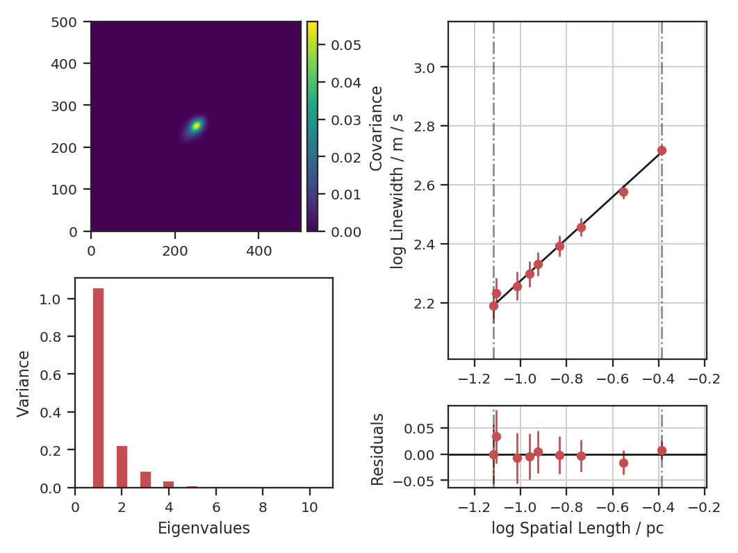
Since the correction is not linear, the slope changes with the beam correction. If the header of the data has the beam information defined, it will be automatically read in and beam_fwhm will not have to be given.
Both of the PCA runs above do not subtract the mean of the data before creating the covariance matrix. Technically, this is not how PCA is defined (see Overview above) and the decomposition is not performed on a true covariance matrix. The justification used in Brunt & Heyer 2002a and Brunt & Heyer 2002b is that the mean has a physical meaning in this case: it’s the largest spatial scale across the map. If we do subtract the mean, how does this affect the index?
>>> pca.run(verbose=True, min_eigval=1e-4, spatial_output_unit=u.pc,
...         spectral_output_unit=u.m / u.s, brunt_beamcorrect=True,
...         beam_fwhm=10 * u.arcsec, mean_sub=True)  # doctest: +SKIP
Proportion of Variance kept: 0.9998085325029037
Index: 0.86 (0.83, 0.89)
Gamma: 1.12 (0.72, 1.53)
Sonic length: 3.947e+00 (3.107e+00, 4.787e+00) pix at 10.0 K
The plot shows how the structure of the covariance matrix has changed. There remains a central peak, though it is smaller, and the positive structure around it is more elongated. The bar plot shows that the relative values of the eigenvalues have changed significantly; this intuitively makes sense as the covariance structure was changed. The index measured is significantly higher than the 0.71 measured above. If we compare the points on the size-line width relation, we see that the steeper relation results from the spectral width remaining the same as in the the non-mean subtracted case, while the spatial size is decreased.
The default setting is to not subtract the mean in order to best reproduce the established Brunt & Heyer formalism. This comparison is included to demonstrate its effect and to highlight that, in not subtracting the mean, some of the assumptions used in PCA are violated. See the PCA Wikipedia page for more information.
The run command has several steps hidden within it. To demonstrate the whole process, the individual steps are broken down below. There are 4 major steps: decomposition, spatial fitting, spectral fitting, and fitting of the size-line width relation.
First, the eigenvalue decomposition is performed using compute_pca:
>>> pca.compute_pca(mean_sub=False, n_eigs='auto', min_eigval=1e-4, eigen_cut_method='value')  # doctest: +SKIP
>>> pca.n_eigs  # doctest: +SKIP
10
mean_sub controls whether to subtract the channel means when calculating the covariance matrix. Formally, this is implied when calculating any covariance matrix, but is not done in the Brunt & Heyer works (see above). n_eigs sets the number of important principal components (which will be used to fit the size-line width relation). This can be an integer, or the code will determine the number of important components based off of a threshold given in min_eigval. When eigen_cut_method='value', min_eigval is the smallest eigenvalue to consider important. Since the variance is related to the level of variance due to noise in the data, it is practical to set this to a few times the noise variance. When eigen_cut_method='proportion', min_eigval now corresponds to the total proportion of variance that is considered important:
>>> pca.compute_pca(mean_sub=False, n_eigs='auto', min_eigval=0.99, eigen_cut_method='proportion')  # doctest: +SKIP
>>> pca.n_eigs  # doctest: +SKIP
4
This will keep the number of components that describe 99% of the variance in the data. The percentage of variance described by a principal component is its eigenvalue divided by the sum of all eigenvalues (the total variance in the data). All other components beyond these levels are due to irreducible noise. These noise components can be thought of as an N-dimensional sphere, where it becomes impossible to diminish the remaining variance as there is no preferred direction.
The eigenvalues of the important components can be generated with:
>>> pca.eigvals # doctest: +SKIP
This will return the full set of eigenvalues as a two-dimensional array with a shape equal to the number of spectral channels in the data. To only return the important eigenvalues, use:
>>> pca.eigvals[:, :pca.n_eigs] # doctest: +SKIP
Eigenimages have the same shape as the spatial dimensions of the data. To save memory, eigenimages are not cached and are calculated from the data and set of eigenvalues:
>>> eigimgs = pca.eigimages() # doctest: +SKIP
eigimgs is a three-dimensional array, with two spatial axes and the third the number of eigenimages requested. By default, the number of eigenimages returned is equal to pca.n_eigs. To instead return the first n eigenimages:
>>> n = 40
>>> eigimgs = pca.eigimages(n)  # doctest: +SKIP
The second step is to calculate the spatial size scales from the autocorrelation of the eigenimages (reverting back to the PCs from eigen_cut_method='value'):
>>> pca.compute_pca(mean_sub=False, n_eigs='auto', min_eigval=1e-4,
...                 eigen_cut_method='value')  # doctest: +SKIP
>>> pca.find_spatial_widths(method='contour', beam_fwhm=10 * u.arcsec,
...                         brunt_beamcorrect=True, diagnosticplots=True)  # doctest: +SKIP
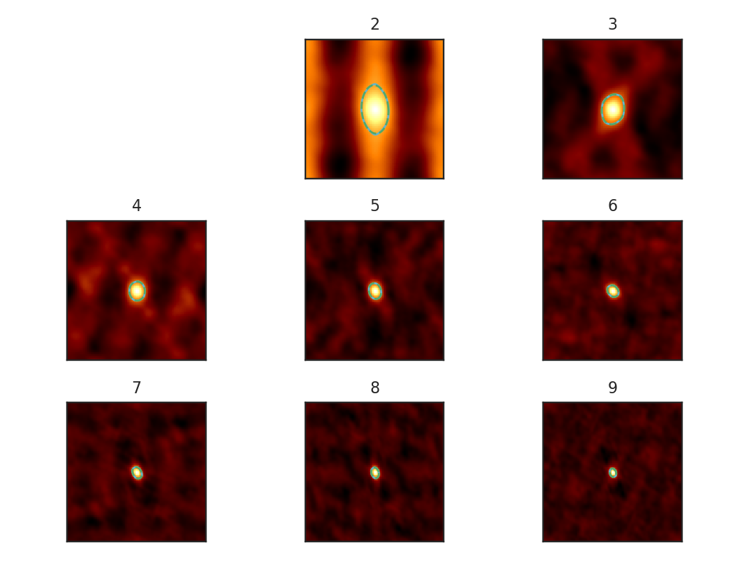
This will find the spatial widths by fitting an ellipse to the 1/e contour about the peak in the autocorrelation image, following the fitting technique described by Brunt & Heyer. The first 9 autocorrelation images are shown in the above image, where the cyan contours are the true 1/e contour, and the green dashed line is the elliptical fit. Note that the first autocorrelation image is not shown. This is because the fitting routine failed; if the 1/e level is not reached in the data, there is no contour to fit to. This means that the largest spatial scale in the data (which critically depends on the mean) is larger than the spatial size of the data. For a periodic-box simulation, which this example data is produced from, it is not surprising that this has occurred. Note: If this issue is encountered in observational data (or anything without periodic boundaries), try padding the data cube in the spatial directions with zeros to simulate a larger map size.
method may also be set to fit to fit a 2D Gaussian to the peak, interpolate which estimates the 1/e from the peak using a fine grid about the peak region, and xinterpolate which first fits a 2D Gaussian to better determine the fine grid to use in interpolation. The default method is contour.
When beam correction is applied (brunt_beamcorrect), the angular FWHM of the beam is needed. This is to deconvolve the spatial widths with the beam size. Note that all spatial scales that cannot be deconvolved from the beam will be set to NaN. If the BMAJ keyword is set in the FITS header in cube, this will be read automatically (also if the radio_beam package is installed, a few other keywords will be recognized). Otherwise, this must be specified in beam_fwhm. If the data do not have a beam size, brunt_beamcorrect=False will need to be specified in find_spatial_widths and run.
Third, we find the spectral widths:
>>> pca.find_spectral_widths(method='walk-down')  # doctest: +SKIP
>>> autocorr_spec = pca.autocorr_spec()  # doctest: +SKIP
>>> x = np.fft.rfftfreq(500) * 500  # doctest: +SKIP
>>> fig, axes = plt.subplots(3, 3, sharex=True, sharey=True)  # doctest: +SKIP
>>> for i, ax in zip(range(9), axes.ravel()):  # doctest: +SKIP
>>>     ax.plot(x, autocorr_spec[:251, i])  # doctest: +SKIP
>>>     ax.axhline(np.exp(-1), label='exp(-1)', color='r', linestyle='--')  # doctest: +SKIP
>>>     ax.axvline(pca.spectral_width(u.pix)[i].value,
...                label='Fitted Width', color='g', linestyle='-.')  # doctest: +SKIP
>>>     ax.set_title("{}".format(i + 1))  # doctest: +SKIP
>>>     ax.set_xlim([0, 50])  # doctest: +SKIP
>>>     if i == 0:  # doctest: +SKIP
>>>         ax.legend()  # doctest: +SKIP
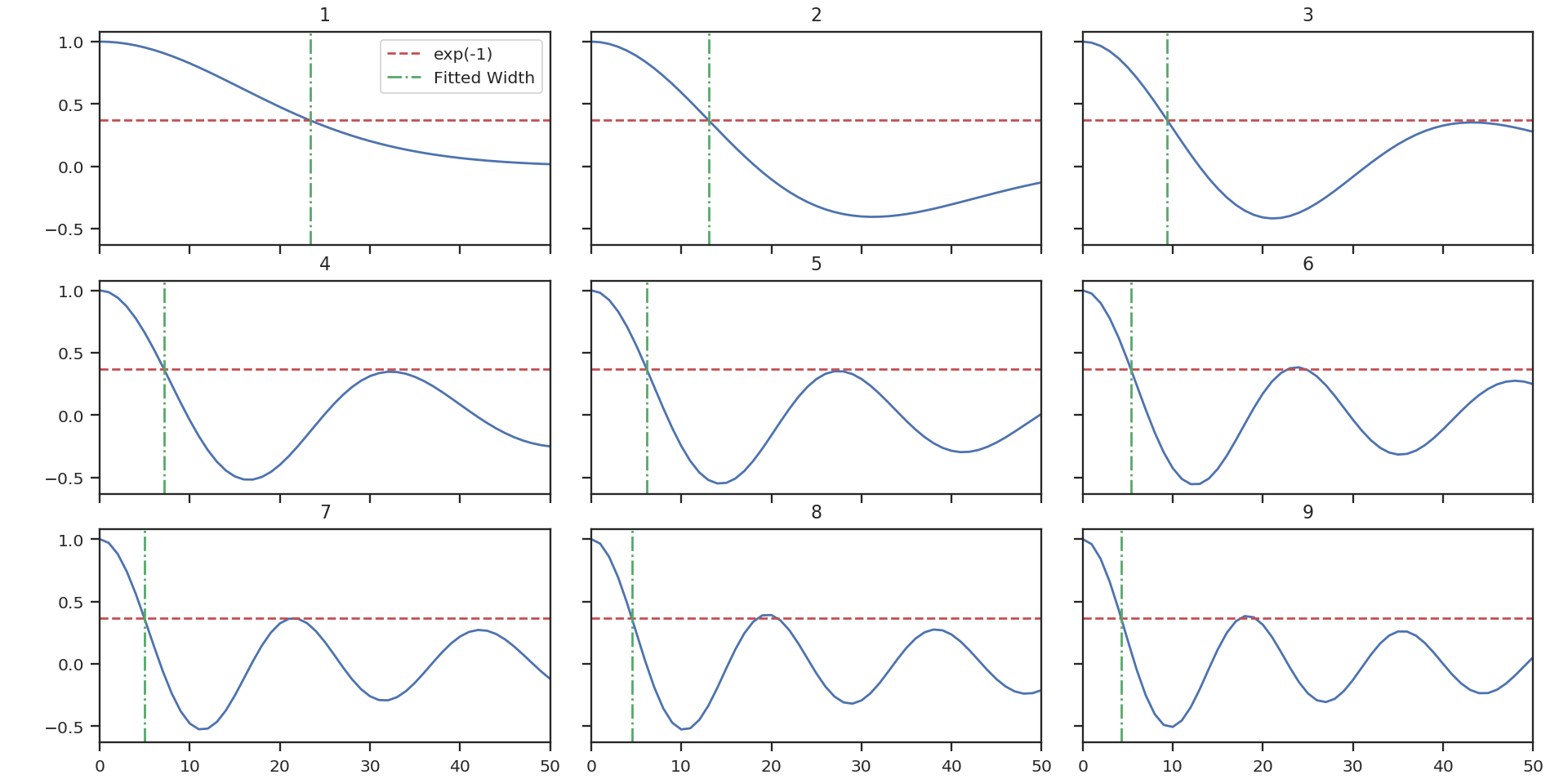
The above image shows the 50 components of the first 9 autocorrelation spectra (the data cube has 500 channels in total, but this is the region of interest). The local minima referred to in the next paragraph are the first minimum points in each of the spectra.
There are three methods available to estimate spectral widths of the autocorrelation spectra. walk-down starts from the peak and continues until the 1/e level is reached. The width is estimated by averaging the points before and after this level is reached. This is the method used by Brunt & Heyer. Otherwise, method may be set to fit, which fits a Gaussian to the data before the first local minimum occurs, and interpolate, which does the same, but through interpolating onto a finer grid. As shown in the above figure, the number of oscillations in the autocorrelation spectrum increases with the Nth principal component. The width of interest is determined from the first peak to the first minimum.
Note: If your input data have few spectral channels, it may be necessary to pad additional channels of zeros onto the data. Otherwise the 1/e level may not be reached. This should not have a significant effect on the results, as the added eigenvalues of these channels will be zero and should not be considered.
Finally, we fit the size-line width relation. There is no clear independent variable to fit, and significant errors in both dimensions which must be taken into account. This is the error-in-variables problem, and an excellent explanation is provided in Hogg, Bovy & Lang 2010. The Brunt & Heyer works have used the bisector method. In TurbuStat, two fitting methods are available: Orthogonal Distance Regression (ODR), and a Markov Chain Monte Carlo (MCMC) method. Practically both methods are doing the same thing, but the MCMC provides a direct sampling (assuming uniform priors). The MCMC method requires the emcee package to be installed.
To run ODR:
>>> pca.fit_plaw(fit_method='odr', verbose=True) # doctest: +SKIP
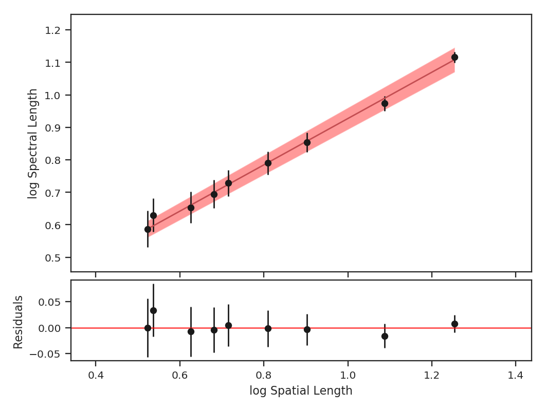
And to run the MCMC:
>>> pca.fit_plaw(fit_method='bayes', verbose=True) # doctest: +SKIP
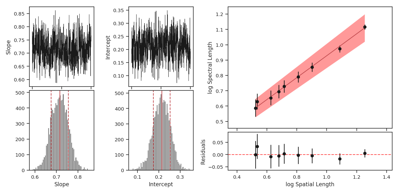
Additional arguments for setting the chain properties can be passed as well. See documentation for bayes_linear. The verbose mode shows the fit results along with the data points.
The interesting outputs from this analysis are estimates of the slopes of the size-line width relation (\(\gamma\)) and the sonic length:
>>> pca.gamma  # doctest: +SKIP
0.897
>>> pca.sonic_length(T_k=10 * u.K, mu=1.36, unit=u.pc)  # doctest: +SKIP
(<Quantity 0.10021154 pc>, <Quantity [0.09024886, 0.111332  ] pc>)
Sonic length is defined as the length at which the fitted line intersects the sounds speed (temperature can be specified with T_k above). Since the sonic length depends on temperature and \(\mu\), this is a function and not a property like \(\gamma\). PCA.sonic_length also returns the 1-sigma error bounds. The error bounds in \(\gamma\) can be accessed with PCA.gamma_error_range.
PDF
Overview
A common technique used in ISM and molecular cloud studies is measurement of the shape of the probability density function (PDF). Often, column density or extinction values are used to construct the PDF. Intensities may also be used, but may be subject to more severe optical depth effects. Properties of the PDF, when related to an analytical form, have been found to correlate with changes in the turbulent properties (e.g., Kowal et al. 2007, Federrath et al. 2010) and gravity (e.g., Burkhart et al. 2015, Burkhart et al. 2017).
A plethora of papers are devoted to this topic, and there is much debate over the form of these PDFs (Lombardi et al. 2015). TurbuStat’s implementation seeks to be flexible because of this. Parametric and non-parametric measures to describe PDFs are shown below.
Using
The data in this tutorial are available here.
We need to import the PDF code, along with a few other common packages:
>>> from turbustat.statistics import PDF
>>> from astropy.io import fits
Since the PDF is a one-dimensional view of the data, any dimension data can be passed. For this tutorial, we will use the zeroth moment (integrated intensity):
>>> moment0 = fits.open("Design4_flatrho_0021_00_radmc_moment0.fits")[0]  # doctest: +SKIP
>>> pdf_mom0 = PDF(moment0, min_val=0.0, bins=None)  # doctest: +SKIP
>>> pdf_mom0.run(verbose=True)  # doctest: +SKIP
Optimization terminated successfully.
         Current function value: 6.007851
         Iterations: 34
         Function evaluations: 69
                              Likelihood Results
==============================================================================
Dep. Variable:                      y   Log-Likelihood:                -98433.
Model:                     Likelihood   AIC:                         1.969e+05
Method:            Maximum Likelihood   BIC:                         1.969e+05
Date:                Sun, 16 Jul 2017
Time:                        15:06:22
No. Observations:               16384
Df Residuals:                   16382
Df Model:                           2
==============================================================================
                 coef    std err          z      P>|z|      [0.025      0.975]
------------------------------------------------------------------------------
par0           0.4360      0.002    181.019      0.000       0.431       0.441
par1         225.6771      0.769    293.602      0.000     224.171     227.184
==============================================================================

The resulting PDF and ECDF of the data are plotted, along with a log-normal fit to the PDF. ECDF is the empirical cumulative distribution function defined as the cumulative sum of the data. By default, PDF will fit a log-normal to the PDF. Choosing other models and disabling the fitting are discussed below.
The fit parameters can be accessed from model_params and the standard errors from model_stderrs. The fitting in PDF uses the stats distributions. The scipy implementation for a log-normal defines the two fit parameters as par0 = exp(mu) and par1 = sigma.
There are several options that can be set. Using min_val will set the lower limit on values to consider in the PDF. bins allows a custom array of bins (edges) to be given. By default, the bins are of equal width, with the number set by the square root of the number of data points (a good estimate when the number of samples is >100).
With the ECDF calculated, we can check the percentile of different values in the data:
>>> pdf_mom0.find_percentile(500)  # doctest: +SKIP
96.3134765625
Or if we want to find the value at a certain percentile:
>>> pdf_mom0.find_at_percentile(96.3134765625)  # doctest: +SKIP
499.98911349468841
The values are not exact between the two operations because the ECDF function was computed with finite values. Note that brightness unit conversions are not yet supported and data values should be passed as floats.
If an array of the uncertainties is available, these may be passed as weights:
>>> moment0_err = fits.open("Design4_flatrho_0021_00_radmc_moment0.fits")[1]  # doctest: +SKIP
>>> pdf_mom0 = PDF(moment0, min_val=0.0, bins=None, weights=moment0_error.data**-2)  # doctest: +SKIP
>>> pdf_mom0.run(verbose=True)  # doctest: +SKIP
Optimization terminated successfully.
         Current function value: 8.470342
         Iterations: 43
         Function evaluations: 86
                              Likelihood Results
==============================================================================
Dep. Variable:                      y   Log-Likelihood:            -1.3878e+05
Model:                     Likelihood   AIC:                         2.776e+05
Method:            Maximum Likelihood   BIC:                         2.776e+05
Date:                Sun, 16 Jul 2017
Time:                        15:06:23
No. Observations:               16384
Df Residuals:                   16382
Df Model:                           2
==============================================================================
                 coef    std err          z      P>|z|      [0.025      0.975]
------------------------------------------------------------------------------
par0           0.4468      0.002    181.019      0.000       0.442       0.452
par1        2584.0353      9.019    286.499      0.000    2566.358    2601.713
==============================================================================
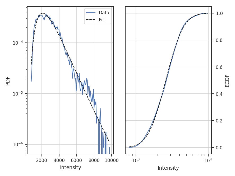
Since the data are now defined as data / stderr^2, the fit parameters have changed. While this scaling makes it difficult to use the fit parameters to compare with theoretical preductions, it can be useful when comparing data sets non-parametrically.
When comparing to the PDFs from other data, adopting a common normalization scheme can aid in highlighting similarities and differences. The four normalizations that can be set with normalization_type are demonstrated below. Adopting different normalizations highlights different portions of the data, making it important to choose a normalization appropriate for the data. Each of these normalizations subtly makes assumptions on the data’s properties. Note that fitting is disabled here since some of the normalization types scale the data to negative values and cannot be fit with a log-normal distribution.
standardize subtracts the mean and divides by the standard deviation; this is appropriate for normally-distributed data:
>>> pdf_mom0 = PDF(moment0, normalization_type='standardize')  # doctest: +SKIP
>>> pdf_mom0.run(verbose=True, do_fit=False)  # doctest: +SKIP
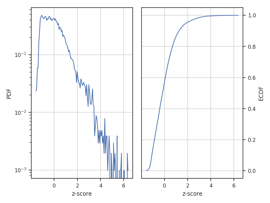
center subtracts the mean from the data:
>>> pdf_mom0 = PDF(moment0, normalization_type='center')  # doctest: +SKIP
>>> pdf_mom0.run(verbose=True, do_fit=False)  # doctest: +SKIP
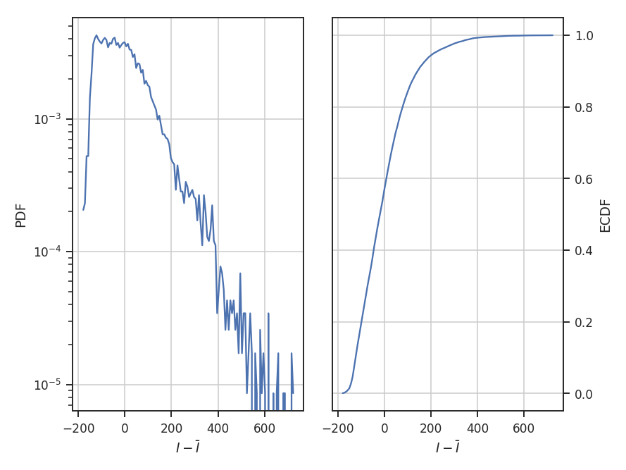
normalize subtracts the minimum in the data and divides by the range in the data, thereby scaling the data between 0 and 1:
>>> pdf_mom0 = PDF(moment0, normalization_type='normalize')  # doctest: +SKIP
>>> pdf_mom0.run(verbose=True, do_fit=False)  # doctest: +SKIP
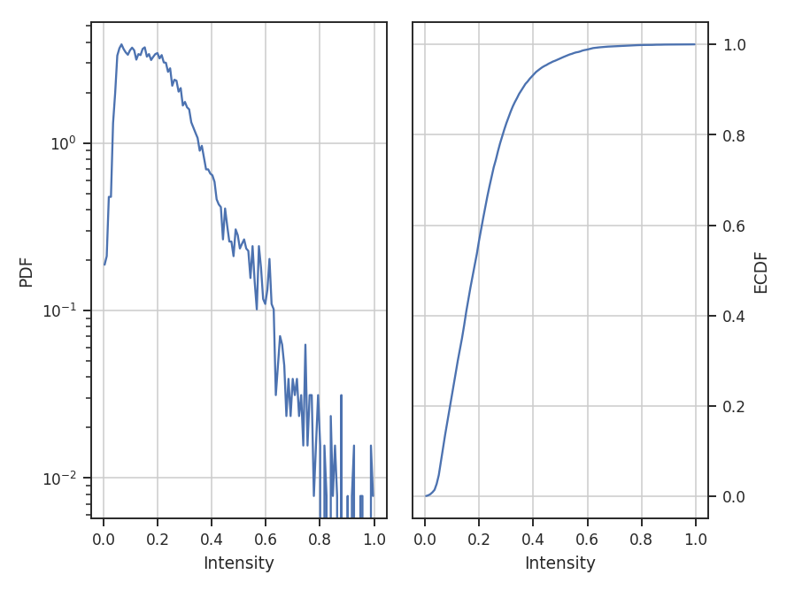
normalize_by_mean divides the data by its mean. This is the most common normalization found in the literature on PDFs since the commonly used parametric forms (log-normal and power-laws) can be arbitrarily scaled by the mean.
>>> pdf_mom0 = PDF(moment0, normalization_type='normalize_by_mean')  # doctest: +SKIP
>>> pdf_mom0.run(verbose=True, do_fit=False)  # doctest: +SKIP
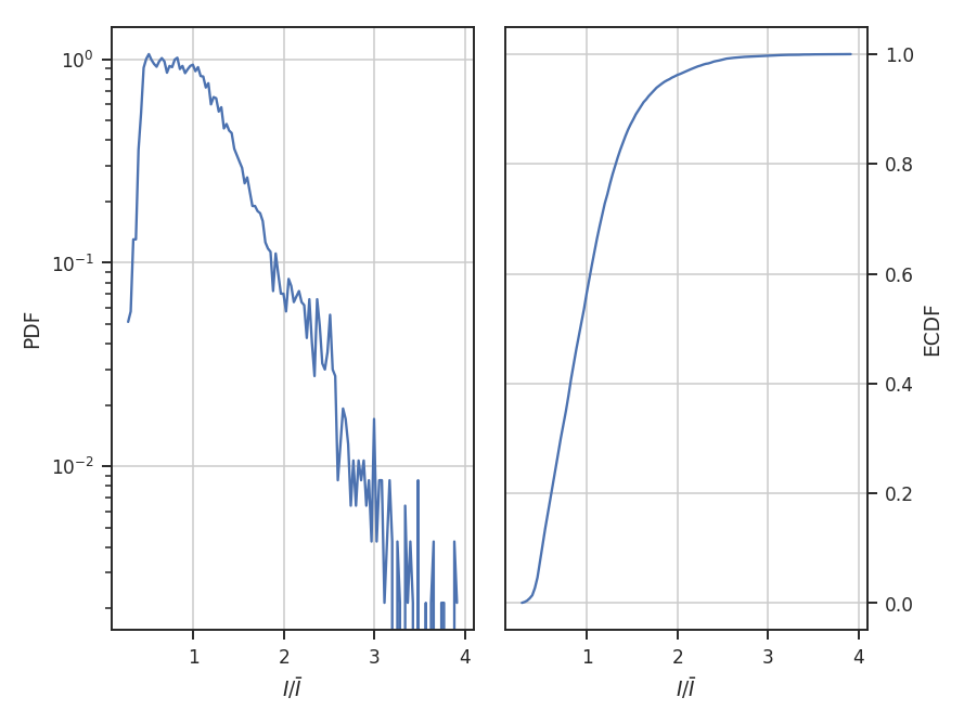
The example data are well-described by a log-normal, making the normalization by the mean an appropriate choice. Note how the shape of the distribution appears unchanged in these examples, but the axis they’re defined on changes.
The distribution fitting shown above uses a maximum likelihood estimate (MLE) to find the parameter values and their uncertainties. This works well for well-behaved data, like those used in this tutorial, where the parametric description fits the data well. When this is not the case, the standard errors can be extremely under-estimated. One solution is to adopt a Monte Carlo approach for fitting. When the emcee package is installed, fit_pdf will fit the distribution using MCMC. Note that all keyword arguments to fit_pdf can also be passed to run.
>>> pdf_mom0 = PDF(moment0, min_val=0.0, bins=None)  # doctest: +SKIP
>>> pdf_mom0.run(verbose=True, fit_type='mcmc')  # doctest: +SKIP
Ran chain for 2000 iterations
Used 20 walkers
Mean acceptance fraction of 0.722775
Parameter values: [   0.43589657  225.69177379]
15th to 85th percentile ranges: [ 0.00498541  1.51322986]
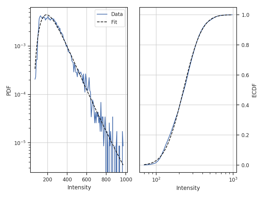
The MCMC fit finds the same parameter values (see the first example above) with a ~1-sigma range about twice that of the MLE fit. The MCMC chain is ran for 200 burn-in steps, followed by 2000 steps that are used to estimate the distribution parameters. These can be altered by passing burnin and steps to the run command above. Other accepted keywords can be found in the emcee documentation.
Warning
MCMC results should not be blindly accepted. It is important to check the behaviour of the chain to ensure it converged and has adequately explored the parameter space around the converged result.
To check if the MCMC has converged, a trace plot of parameter value versus step in the chain can be made:
>>> pdf_mom0.trace_plot()
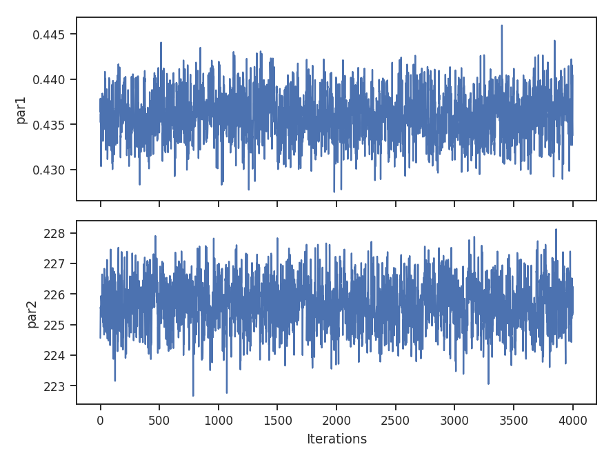
We can also look at the sample distributions for each fit parameter using a corner plot. This requires the corner.py package to be installed.
>>> pdf_mom0.corner_plot() # doctest: +SKIP
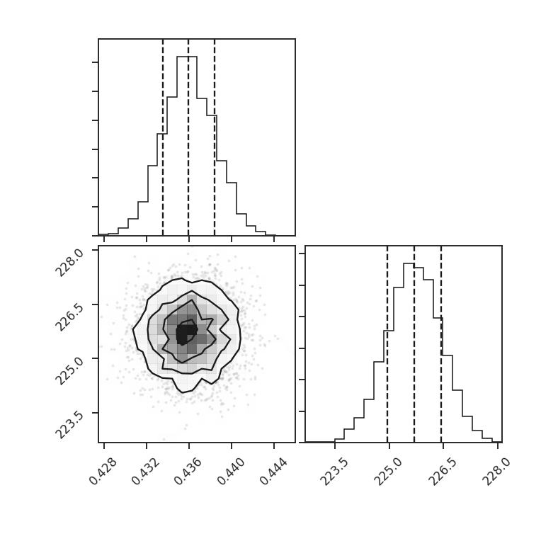
Each parameter distribution is showed (1D histograms) and their interaction (2D histogram), which is useful for exploring covariant parameters in the fit. The dotted lines show the 16th, 50th, and 84th quantiles. Each of the distributions here is close to normally-distributed and appears well-behaved.
The log-normal distribution is typically not used for observational data since low column densities or extinction regions have greater uncertainties and/or are incompletely sampled in the data (see Lombardi et al. 2015). A power-law model may be a better model choice in this case. We can choose to fit other models by passing different rv_continuous models to model in run. Note that the fit will fail if the data are outside of the accepted range for the given model (such as negative values for the log-normal distribution).
For this example, let us consider values below 250 K m/s to be unreliable. We will fit a pareto distribution to the integrated intensities above this (the scipy powerlaw model requires a positive index).
>>> import scipy.stats as stats  # doctest: +SKIP
>>> plaw_data = stats.pareto.rvs(2, size=5000)  # doctest: +SKIP
>>> pdf_mom0 = PDF(moment0, min_val=250.0, normalization_type=None)  # doctest: +SKIP
>>> pdf_mom0.run(verbose=True, model=stats.pareto,
...              fit_type='mle', floc=False)  # doctest: +SKIP
Optimization terminated successfully.
         Current function value: 5.641058
         Iterations: 84
         Function evaluations: 159
Fitted parameters: [   3.27946996   -0.58133183  250.61486355]
Covariance calculation failed.
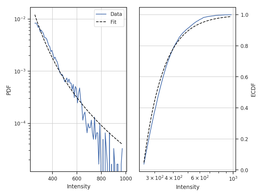
Based on the deviations in the ECDF plot, the log-normal fit was better for this data, though the power-law does adequately describe the data at high integrated intensities. But, there are issues with the fit. The MLE routine diverges when calculating the covariance matrix and standard errors. There are important nuances for fitting heavy-tailed distributions that are not included in the MLE fitting here. See the powerlaw package for the correct approach.
Note that an additional parameter, floc, has been set. This stops the loc parameter from being fixed in the fit, which is appropriate for the default fitting of a log-normal distribution. The scale parameter can similarly be fixed with fscale. See the scipy.stats documentation for an explanation of these parameters.
All of these examples use the zeroth moment from the data. Since PDFs are equally valid for any dimension of data, we can also find the PDF for the PPV cube. The class and function calls are identical:
>>> from spectral_cube import SpectralCube
>>> cube = SpectralCube.read("Design4_flatrho_0021_00_radmc.fits")[0]  # doctest: +SKIP
>>> pdf_cube = PDF(cube).run(verbose=True, do_fit=False)  # doctest: +SKIP
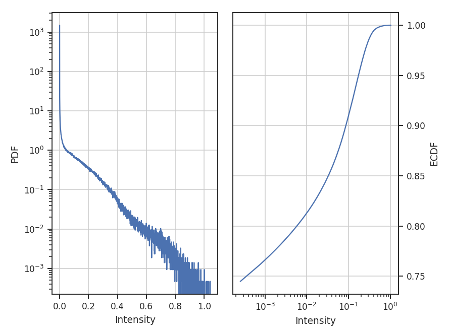
References
As stated above, there are a ton of papers measuring properties of the PDF. Below are just a few examples with different PDF uses and discussions:
Spatial Power Spectrum
Overview
A common analysis technique for two-dimensional images is the spatial power spectrum – the square of the 2D Fourier transform of an image. A radial profile of the 2D power spectrum gives the 1D power spectrum. The slope of this 1D spectrum can be compared to the expected indices in different physical limits. For example, the velocity field of Kolmogorov turbulence follows \(k^{-5/3}\), while Burgers’ turbulence has \(k^{-2}\).
However, observations are a combination of both velocity and density fluctuations (e.g., Lazarian & Pogosyan 2000), and the measured index from an integrated intensity map depend on both components, as well as optical depth effects. For a turbulent optically thin tracer, an integrated intensity image (or zeroth moment) will have \(k^{-11/3}\), while an optically thick tracer saturates to \(k^{-3}\) (Lazarian & Pogosyan 2004, Burkhart et al. 2013). The effect of velocity resolution is discussed in the VCA tutorial.
Using
The data in this tutorial are available here.
We need to import the PowerSpectrum code, along with a few other common packages:
>>> from turbustat.statistics import PowerSpectrum
>>> from astropy.io import fits
And we load in the data:
>>> moment0 = fits.open("Design4_flatrho_0021_00_radmc_moment0.fits")[0] # doctest: +SKIP
The power spectrum is computed using:
>>> pspec = PowerSpectrum(moment0, distance=250 * u.pc)  # doctest: +SKIP
>>> pspec.run(verbose=True, xunit=u.pix**-1)  # doctest: +SKIP
                            OLS Regression Results
==============================================================================
Dep. Variable:                      y   R-squared:                       0.941
Model:                            OLS   Adj. R-squared:                  0.941
Method:                 Least Squares   F-statistic:                     1426.
Date:                Fri, 29 Sep 2017   Prob (F-statistic):           1.44e-56
Time:                        14:32:47   Log-Likelihood:                -52.829
No. Observations:                  91   AIC:                             109.7
Df Residuals:                      89   BIC:                             114.7
Df Model:                           1
Covariance Type:            nonrobust
==============================================================================
                 coef    std err          t      P>|t|      [0.025      0.975]
------------------------------------------------------------------------------
const          3.1677      0.103     30.828      0.000       2.964       3.372
x1            -5.0144      0.133    -37.761      0.000      -5.278      -4.751
==============================================================================
Omnibus:                        3.532   Durbin-Watson:                   0.129
Prob(Omnibus):                  0.171   Jarque-Bera (JB):                3.481
Skew:                          -0.468   Prob(JB):                        0.175
Kurtosis:                       2.797   Cond. No.                         4.40
==============================================================================
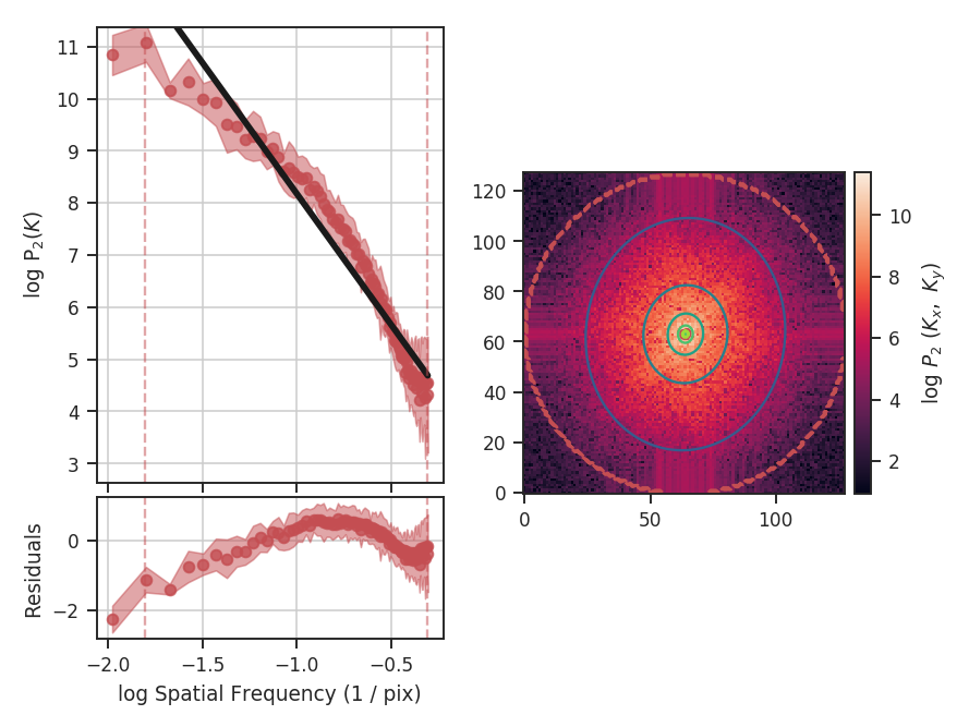
The code returns a summary of the one-dimensional fit and a figure showing the one-dimensional spectrum and model on the left, and the two-dimensional power-spectrum on the right. If fit_2D=True is set in run (the default setting), the contours on the two-dimensional power-spectrum are fit using an elliptical power-law model. The dashed red lines (or contours) on both plots are the limits of the data used in the fits. We use an elliptical power-law model:
Here, the power-law index is \(\Gamma\), the orientation angle of the ellipse with respect to the \(x,y\) coordinate system is given by \(\theta\) and the ellipticity is \(q\in [0,1)\).
The power spectrum of this simulation has a slope of \(-3.3\pm0.1\), but the power-spectrum deviates from a single power-law on small scales. This is due to the the limited inertial range in this simulation. The spatial frequencies used in the fit can be limited by setting low_cut and high_cut. The inputs should have frequency units in pixels, angle, or physical units. For example,
>>> pspec.run(verbose=True, xunit=u.pix**-1, low_cut=0.025 / u.pix,
...           high_cut=0.1 / u.pix)  # doctest: +SKIP
                            OLS Regression Results
==============================================================================
Dep. Variable:                      y   R-squared:                       0.971
Model:                            OLS   Adj. R-squared:                  0.968
Method:                 Least Squares   F-statistic:                     398.6
Date:                Thu, 28 Sep 2017   Prob (F-statistic):           1.42e-10
Time:                        17:02:20   Log-Likelihood:                 14.077
No. Observations:                  14   AIC:                            -24.15
Df Residuals:                      12   BIC:                            -22.87
Df Model:                           1
Covariance Type:            nonrobust
==============================================================================
                 coef    std err          t      P>|t|      [0.025      0.975]
------------------------------------------------------------------------------
const          5.5109      0.190     29.021      0.000       5.097       5.925
x1            -3.0223      0.151    -19.964      0.000      -3.352      -2.692
==============================================================================
Omnibus:                        0.901   Durbin-Watson:                   2.407
Prob(Omnibus):                  0.637   Jarque-Bera (JB):                0.718
Skew:                          -0.215   Prob(JB):                        0.698
Kurtosis:                       1.977   Cond. No.                         15.2
==============================================================================

When limiting the fit to the inertial range, the slope is \(-3.0\pm0.2\). low_cut and high_cut can also be given as spatial frequencies in angular units (e.g., u.deg**-1). And since a distance was specified, the low_cut and high_cut can also be given in physical frequency units (e.g., u.pc**-1).
The fit to the two-dimensional power-spectrum has also changed. These parameters aren’t included in the fit summary for the 1D fit. Instead, they can be accessed through:
>>> print(pspec.slope2D, pspec.slope2D_err)  # doctest: +SKIP
(-3.155235947194412, 0.19744198375014044)
>>> print(pspec.ellip2D, pspec.ellip2D_err)  # doctest: +SKIP
(0.74395734515060385, 0.043557506230624203)
>>> print(pspec.theta2D, pspec.theta2D_err)  # doctest: +SKIP
(1.1364954648370515, 0.09436799399259721)
The slope is moderately steeper than in the 1D model, but within the respective uncertainty ranges. By default, the parameter uncertainties for the 2D model are determined by a bootstrap. After fitting the model, the residuals are resampled and added back to the data. The resampled data are then fit to the model. This procedure is repeated some number of times (the default is 100) to build up distributions for the fit parameters. The bootstrap estimation is enabled in the code by setting the bootstrap keyword to True in fit_2Dpspec and the number of iterations is set with niters (the default is 100). These can be set in run by passing a keyword dictionary to fit_2D_kwargs (e.g., fit_2D_kwargs={'bootstrap': False}). The other parameters are the ellipticity, which is bounded between 0 and 1 (with 1 being circular), and theta, the angle between the x-axis and the semi-major axis of the ellipse. Theta is bounded between 0 and \(\pi\). The 2D power spectrum here is moderately anisotropic.
Breaks in the power-law behaviour in observations (and higher-resolution simulations) can result from differences in the physical processes dominating at those scales (e.g., Swift & Welch 2008). To capture this behaviour, PowerSpectrum can be passed a break point to enable fitting with a segmented linear model (Lm_Seg):
>>> pspec = PowerSpectrum(moment0, distance=250 * u.pc)  # doctest: +SKIP
>>> pspec.run(verbose=True, xunit=u.pc**-1, low_cut=0.02 / u.pix, high_cut=0.4 / u.pix,
...           fit_kwargs={'brk': 0.1 / u.pix, 'log_break': False}, fit_2D=False)  # doctest: +SKIP
                            OLS Regression Results
==============================================================================
Dep. Variable:                      y   R-squared:                       0.996
Model:                            OLS   Adj. R-squared:                  0.995
Method:                 Least Squares   F-statistic:                     4904.
Date:                Fri, 29 Sep 2017   Prob (F-statistic):           1.84e-77
Time:                        14:29:10   Log-Likelihood:                 61.421
No. Observations:                  70   AIC:                            -114.8
Df Residuals:                      66   BIC:                            -105.8
Df Model:                           3
Covariance Type:            nonrobust
==============================================================================
                 coef    std err          t      P>|t|      [0.025      0.975]
------------------------------------------------------------------------------
const          5.1169      0.087     59.057      0.000       4.944       5.290
x1            -3.3384      0.082    -40.924      0.000      -3.501      -3.176
x2            -4.9624      0.191    -26.043      0.000      -5.343      -4.582
x3            -0.0084      0.048     -0.174      0.863      -0.105       0.088
==============================================================================
Omnibus:                        3.812   Durbin-Watson:                   1.096
Prob(Omnibus):                  0.149   Jarque-Bera (JB):                2.211
Skew:                          -0.191   Prob(JB):                        0.331
Kurtosis:                       2.218   Cond. No.                         22.4
==============================================================================
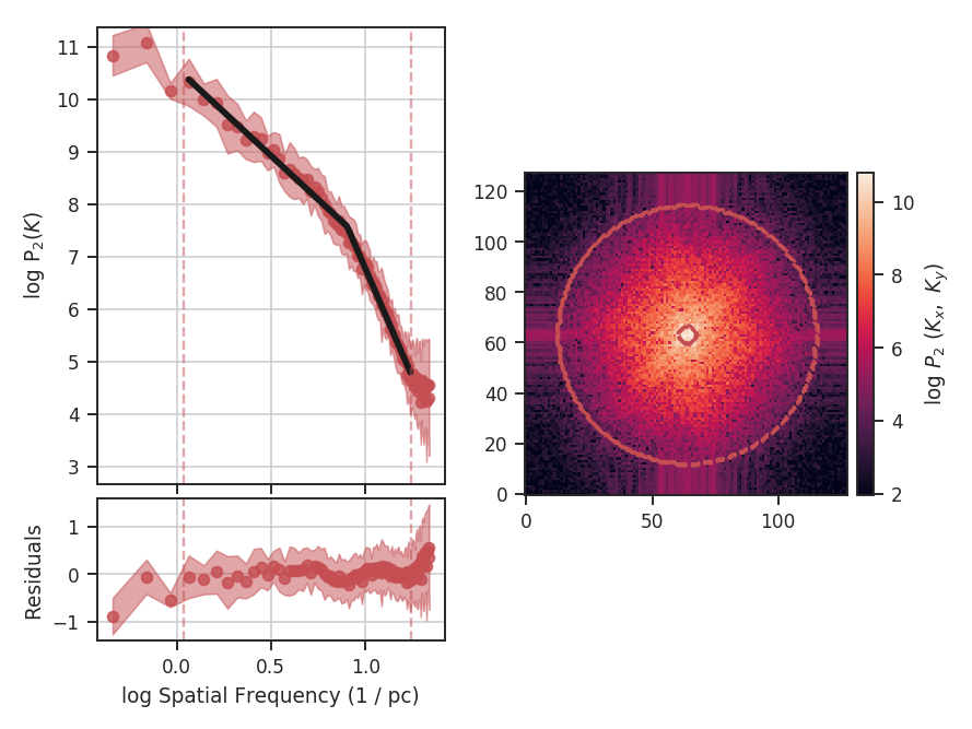
brk is the initial guess for where the break point location is. Here I’ve set it to the extent of the inertial range of the simulation. log_break should be enabled if the given brk is already the log (base-10) value (since the fitting is done in log-space). The segmented linear model iteratively optimizes the location of the break point, trying to minimize the gap between the different components. This is the x3 parameter above. The slopes of the components are x1 and x2, but the second slope is defined relative to the first slope (i.e., if x2=0, the slopes of the components would be the same). The true slopes can be accessed through pspec.slope and pspec.slope_err. The location of the fitted break point is given by pspec.brk, and its uncertainty pspec.brk_err. If the fit does not find a good break point, it will revert to a linear fit without the break.
Note that the 2D fitting was disabled in this last example. The 2D model cannot fit a break point, and will instead try to fit a single power-law for the between low_cut and high_cut, which we know already know is the wrong model. Thus, it has been disabled to avoid confusion. A strategy for fitting the 2D model when the spectrum shows a break is to first fit the 1D model, find the break point, and then fit the 2D spectrum independently using the break point as the high_cut in fit_2Dpspec.
There may be cases where you want to limit the azimuthal angles used to create the 1D averaged power-spectrum. This may be useful if, for example, you want to find a measure of anistropy but the 2D power-law fit is not performing well. We will add extra constraints to the previous example with a break point:
>>> pspec = PowerSpectrum(moment0, distance=250 * u.pc)  # doctest: +SKIP
>>> pspec.run(verbose=True, xunit=u.pc**-1, low_cut=0.02 / u.pix, high_cut=0.4 / u.pix,
...           fit_2D=False, fit_kwargs={'brk': 0.1 / u.pix, 'log_break': False},
...           radial_pspec_kwargs={"theta_0": 1.13 * u.rad, "delta_theta": 40 * u.deg})  # doctest: +SKIP
                            OLS Regression Results
==============================================================================
Dep. Variable:                      y   R-squared:                       0.990
Model:                            OLS   Adj. R-squared:                  0.989
Method:                 Least Squares   F-statistic:                     2113.
Date:                Fri, 29 Sep 2017   Prob (F-statistic):           1.76e-65
Time:                        14:29:10   Log-Likelihood:                 30.377
No. Observations:                  70   AIC:                            -52.75
Df Residuals:                      66   BIC:                            -43.76
Df Model:                           3
Covariance Type:            nonrobust
==============================================================================
                 coef    std err          t      P>|t|      [0.025      0.975]
------------------------------------------------------------------------------
const          5.7150      0.173     33.005      0.000       5.369       6.061
x1            -2.9371      0.154    -19.041      0.000      -3.245      -2.629
x2            -4.9096      0.254    -19.313      0.000      -5.417      -4.402
x3             0.0156      0.077      0.202      0.840      -0.138       0.169
==============================================================================
Omnibus:                        3.679   Durbin-Watson:                   1.837
Prob(Omnibus):                  0.159   Jarque-Bera (JB):                1.894
Skew:                          -0.030   Prob(JB):                        0.388
Kurtosis:                       2.196   Cond. No.                         22.9
==============================================================================
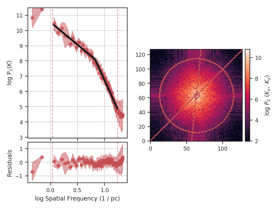
The azimuthal mask has been added onto the plot of the two-dimensional power spectrum. The constraints used here are based on the major axis direction from the two-dimensional fit performed above. This is given as theta_0. The other parameter, delta_theta, is the width of the azimuthal mask to use. Both parameters can be specified in any angular unit.
The default fit uses Ordinary Least Squares. A Weighted Least Squares can be enabled with weighted_fit=True if the segmented linear fit is not used:
>>> pspec = PowerSpectrum(moment0, distance=250 * u.pc)  # doctest: +SKIP
>>> pspec.run(verbose=True, xunit=u.pix**-1, low_cut=0.025 / u.pix, high_cut=0.1 / u.pix,
...           fit_kwargs={'weighted_fit': True})  # doctest: +SKIP
                            WLS Regression Results
==============================================================================
Dep. Variable:                      y   R-squared:                       0.969
Model:                            WLS   Adj. R-squared:                  0.966
Method:                 Least Squares   F-statistic:                     372.0
Date:                Fri, 29 Sep 2017   Prob (F-statistic):           2.13e-10
Time:                        15:08:21   Log-Likelihood:                 13.966
No. Observations:                  14   AIC:                            -23.93
Df Residuals:                      12   BIC:                            -22.65
Df Model:                           1
Covariance Type:            nonrobust
==============================================================================
                 coef    std err          t      P>|t|      [0.025      0.975]
------------------------------------------------------------------------------
const          5.5119      0.194     28.476      0.000       5.090       5.934
x1            -3.0200      0.157    -19.288      0.000      -3.361      -2.679
==============================================================================
Omnibus:                        0.701   Durbin-Watson:                   2.387
Prob(Omnibus):                  0.704   Jarque-Bera (JB):                0.655
Skew:                          -0.235   Prob(JB):                        0.721
Kurtosis:                       2.050   Cond. No.                         15.3
==============================================================================

The fit has not changed significantly but may in certain cases.
If strong emission continues to the edge of the map (and the map does not have periodic boundaries), ringing in the FFT can introduce a cross pattern in the 2D power-spectrum. This effect and the use of apodizing kernels to taper the data is covered here.
Most observational data will be smoothed over the beam size, which will steepen the power spectrum on small scales. To account for this, the 2D power spectrum can be divided by the beam response. This is demonstrated here for spatial power-spectra.
References
Many papers have utilized the power spectrum. An incomplete list is provided below:
Spectral Correlation Function (SCF)
Overview
The Spectral Correlation Function was introduced by Rosolowsky et al. 1999 and Padoan et al. 2001 to quantify the correlation of a spectral-line data cube as a function of spatial separation. There are different forms of the SCF described in the literature (e.g., Padaon et al. 2003). TurbuStat contains the SCF form described in Padaon et al. 2003, which has been used in Yeremi et al. 2014 and Gaches et al. 2015.
\(S(\boldsymbol{\ell})\) is the total correlation between the cube, and the cube shifted by the lag, the vector \(\boldsymbol{\ell}=(\Delta x, \Delta y)\). By repeating this process for a series of \(\Delta x, \Delta y)\) in the spatial dimensions, a 2D correlation surface is created. This surface describes the spatial scales on which the spectral features begin to change.
The correlation surface can be further simplified by computing an azimuthal average, yielding a 1D spectrum of the correlation vs. length of the lag vector. This form, as is presented in Rosolowsky et al. 1999 and Padoan et al. 2001, yields a power-law relation, whose slope can be used to quantify differences between different spectral cubes. An example of this comparison is the study by Gaches et al. 2015, where the effect of chemical species analyzed is traced through changes in the SCF slope.
Using
The data in this tutorial are available here.
Importing a few common packages:
>>> from turbustat.statistics import SCF
>>> from astropy.io import fits
>>> import astropy.units as u
And we load in the data:
>>> cube = fits.open("Design4_flatrho_0021_00_radmc.fits")[0] # doctest: +SKIP
The cube and lags to use are given to initialize the SCF class:
>>> scf = SCF(cube, size=11) # doctest: +SKIP
size describes the total size of one dimension of the correlation surface and will compute the SCF up to a lag of 5 pixels in each direction. Alternatively, a set of custom lag values can be passed using roll_lags (see the example with physical units below). No restriction is placed on the values of these lags, however the azimuthally-averaged spectrum is only usable if the given lags are symmetric with positive and negative values. Also note that lags do not have to be integer values! SCF handles non-integer shifts by shifting the data in the Fourier plane.
To compute the SCF, we run:
>>> scf.run(verbose=True)  # doctest: +SKIP
                            WLS Regression Results
==============================================================================
Dep. Variable:                      y   R-squared:                       0.991
Model:                            WLS   Adj. R-squared:                  0.990
Method:                 Least Squares   F-statistic:                     661.0
Date:                Tue, 18 Jul 2017   Prob (F-statistic):           2.28e-07
Time:                        10:07:56   Log-Likelihood:                 26.958
No. Observations:                   8   AIC:                            -49.92
Df Residuals:                       6   BIC:                            -49.76
Df Model:                           1
Covariance Type:            nonrobust
==============================================================================
                 coef    std err          t      P>|t|      [0.025      0.975]
------------------------------------------------------------------------------
const         -0.0450      0.001    -33.254      0.000      -0.048      -0.042
x1            -0.1624      0.006    -25.710      0.000      -0.178      -0.147
==============================================================================
Omnibus:                        1.340   Durbin-Watson:                   0.445
Prob(Omnibus):                  0.512   Jarque-Bera (JB):                0.696
Skew:                          -0.248   Prob(JB):                        0.706
Kurtosis:                       1.643   Cond. No.                         4.70
==============================================================================

The summary plot shows the correlation surface, a histogram of correlation values, and the 1D spectrum from the azimuthal average, plotted with the power-law fit. A weighted least-squares fit is used to find the slope of the SCF spectrum, where the inverse squared standard deviation from the azimuthal average are used as the weights. The solid contours on the SCF surface are from the 2D fit to the surface, while the blue dot-dashed lines are the extents of the data used in the fit (and match the 1D spectrum limits). See the PowerSpectrum tutorial for a more thorough discussion of the two-dimensional fitting.
The 2D model parameters are not shown in the above summary. Instead, the parameters can be accessed with:
>>> print(scf.slope2D, scf.slope2D_err)  # doctest: +SKIP
(-0.21648274416050342, 0.0029877489213308711)
>>> print(scf.ellip2D, scf.ellip2D_err)  # doctest: +SKIP
(0.89100428375797669, 0.013283231941591638)
>>> print(scf.theta2D, scf.theta2D_err)  # doctest: +SKIP
(0.33117523945671401, 0.06876652735591221)
Since each value in the SCF surface is an average over the whole cube, it tends to be less affected by noise than the power-spectrum based methods (e.g., PowerSpectrum tutorial) and the 2D fit is highly constrained despite having many fewer points to fit. The slope of the 2D model is much steeper than the slope of the 1D model. In the 2D model, the index is defined to be the slope along the minor axis, where the slope is the steepest. The ability to return the slope at any angle will be added to TurbuStat in a future release.
Real data may not have a spectrum described by a single power-law. In this case, the fit limits can be specified using xlow and xhigh to limit which scales are used in the fit.
>>> scf.run(verbose=True, xlow=1 * u.pix, xhigh=5 * u.pix)  # doctest: +SKIP
                            WLS Regression Results
==============================================================================
Dep. Variable:                      y   R-squared:                       0.983
Model:                            WLS   Adj. R-squared:                  0.975
Method:                 Least Squares   F-statistic:                     118.9
Date:                Tue, 18 Jul 2017   Prob (F-statistic):            0.00831
Time:                        10:10:42   Log-Likelihood:                 16.864
No. Observations:                   4   AIC:                            -29.73
Df Residuals:                       2   BIC:                            -30.95
Df Model:                           1
Covariance Type:            nonrobust
==============================================================================
                 coef    std err          t      P>|t|      [0.025      0.975]
------------------------------------------------------------------------------
const         -0.0103      0.010     -1.036      0.409      -0.053       0.032
x1            -0.2027      0.019    -10.902      0.008      -0.283      -0.123
==============================================================================
Omnibus:                          nan   Durbin-Watson:                   2.000
Prob(Omnibus):                    nan   Jarque-Bera (JB):                0.637
Skew:                          -0.020   Prob(JB):                        0.727
Kurtosis:                       1.045   Cond. No.                         10.0
==============================================================================

The one-dimensional power spectrum in the previous examples is averaged over all azimuthal angles. In cases where only a certain range of angles is of interest, limits on the averaged azimuthal angles can be given:
>>> scf.run(verbose=True, xlow=1 * u.pix, xhigh=5 * u.pix,
...         radialavg_kwargs={"theta_0": 1.13 * u.rad,
...                           "delta_theta": 70 * u.deg})  # doctest: +SKIP
                            WLS Regression Results
==============================================================================
Dep. Variable:                      y   R-squared:                       0.987
Model:                            WLS   Adj. R-squared:                  0.981
Method:                 Least Squares   F-statistic:                     157.2
Date:                Mon, 02 Oct 2017   Prob (F-statistic):            0.00630
Time:                        09:00:45   Log-Likelihood:                 17.721
No. Observations:                   4   AIC:                            -31.44
Df Residuals:                       2   BIC:                            -32.67
Df Model:                           1
Covariance Type:            nonrobust
==============================================================================
                 coef    std err          t      P>|t|      [0.025      0.975]
------------------------------------------------------------------------------
const         -0.0067      0.010     -0.695      0.559      -0.048       0.035
x1            -0.2098      0.017    -12.539      0.006      -0.282      -0.138
==============================================================================
Omnibus:                          nan   Durbin-Watson:                   1.899
Prob(Omnibus):                    nan   Jarque-Bera (JB):                0.449
Skew:                          -0.003   Prob(JB):                        0.799
Kurtosis:                       1.358   Cond. No.                         14.4
==============================================================================

theta_0 is the angle at the center of the azimuthal mask and delta_theta is the width of that mask. The mask is shown on the SCF surface by the radial blue-dashed contours.
Here the fit limits were given in pixel units, but angular units and physical units (if a distance is given) can also be passed. For these data, there is some deviation from a power-law at small lags over the range of lags used and so limiting the fitting range has not significantly changed the fit. See Figure 8 in Padoan et al. 2001 for an example of deviations from power-law behaviour in the SCF spectrum.
The slope of the model can be accessed with scf.slope and its standard error with scf.slope_err. The slope and intercept values are in scf.fit.params. scf.fitted_model can be used to evaluate the model at any given lag value. For example:
>>> scf.fitted_model(1 * u.pix)  # doctest: +SKIP
0.97659777310171636
>>> scf.fitted_model(u.Quantity([1, 10]) * u.pix)  # doctest: +SKIP
array([ 0.97659777,  0.61242384])
>>> scf.fitted_model(u.Quantity([50, 100]) * u.arcsec)  # doctest: +SKIP
array([ 0.44197356,  0.3840506 ])
All values passed must have an attached unit. Physical units can be given when a distance has been given (see below).
In some cases, it may be preferable to calculate the SCF on specific physical scales. When SCF is given a distance,
roll_lags, xlow, xhigh, and xunit can be given in physical units. Angular units can always be given, as well, since SCF requires a FITS header. In this example, we will use a set of custom lags in physical units:
>>> distance = 250 * u.pc  # Assume a distance
>>> phys_conv = (np.abs(cube.header['CDELT2']) * u.deg).to(u.rad).value * distance  # doctest: +SKIP
>>> custom_lags = np.arange(-4.5, 5, 1.5) * phys_conv  # doctest: +SKIP
>>> print(custom_lags)  # doctest: +SKIP
[-0.10296379 -0.06864253 -0.03432126  0.          0.03432126  0.06864253 0.10296379] pc
The lags here are equally spaced and centered around zero. phys_conv converts the pixel values into physical units. When calling SCF, the distance must now be given:
>>> scf_physroll = SCF(cube, roll_lags=custom_lags, distance=distance)  # doctest: +SKIP
>>> scf_physroll.run(verbose=True, xunit=u.pc)  # doctest: +SKIP
                            WLS Regression Results
==============================================================================
Dep. Variable:                      y   R-squared:                       0.892
Model:                            WLS   Adj. R-squared:                  0.856
Method:                 Least Squares   F-statistic:                     24.77
Date:                Tue, 18 Jul 2017   Prob (F-statistic):             0.0156
Time:                        10:57:18   Log-Likelihood:                 14.907
No. Observations:                   5   AIC:                            -25.81
Df Residuals:                       3   BIC:                            -26.59
Df Model:                           1
Covariance Type:            nonrobust
==============================================================================
                 coef    std err          t      P>|t|      [0.025      0.975]
------------------------------------------------------------------------------
const         -0.2522      0.038     -6.725      0.007      -0.372      -0.133
x1            -0.1292      0.026     -4.977      0.016      -0.212      -0.047
==============================================================================
Omnibus:                          nan   Durbin-Watson:                   1.495
Prob(Omnibus):                    nan   Jarque-Bera (JB):                0.757
Skew:                           0.914   Prob(JB):                        0.685
Kurtosis:                       2.464   Cond. No.                         19.3
==============================================================================
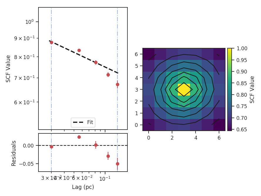
This example takes a bit longer to run than the others because, whenever a non-integer lag is used, the cube is shifted in Fourier space.
Throughout all of these examples, we have assumed that the spatial boundaries can be wrapped. This is appropriate for the example data since they are generated from a periodic-box simulation and is the default setting (boundary='continuous'). Typically this will not be the case for observational data. To avoid wrapping the edges of the data, boundary='cut' can be set to avoid using the portion of the data that has been spatially wrapped:
>>> scf = SCF(cube, size=11)  # doctest: +SKIP
>>> scf.run(verbose=True, boundary='cut')  # doctest: +SKIP
                            WLS Regression Results
==============================================================================
Dep. Variable:                      y   R-squared:                       0.993
Model:                            WLS   Adj. R-squared:                  0.992
Method:                 Least Squares   F-statistic:                     830.7
Date:                Tue, 18 Jul 2017   Prob (F-statistic):           1.16e-07
Time:                        11:13:18   Log-Likelihood:                 24.569
No. Observations:                   8   AIC:                            -45.14
Df Residuals:                       6   BIC:                            -44.98
Df Model:                           1
Covariance Type:            nonrobust
==============================================================================
                 coef    std err          t      P>|t|      [0.025      0.975]
------------------------------------------------------------------------------
const         -0.0834      0.003    -31.106      0.000      -0.090      -0.077
x1            -0.2425      0.008    -28.821      0.000      -0.263      -0.222
==============================================================================
Omnibus:                        0.723   Durbin-Watson:                   0.501
Prob(Omnibus):                  0.697   Jarque-Bera (JB):                0.556
Skew:                          -0.236   Prob(JB):                        0.757
Kurtosis:                       1.797   Cond. No.                         3.38
==============================================================================
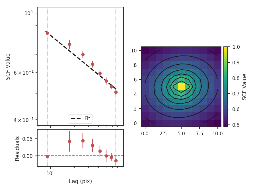
This results in a steeper SCF slope as the edges of the rolled cubes are no longer used.
Computing the SCF can be computationally expensive for moderately-size data cubes. This is due to the need for shifting the entire cube along the spatial dimensions at each lag value. To avoid recomputing the SCF surface, the results of the SCF can be saved as a pickled object:
>>> scf.save_results(output_name="Design4_SCF", keep_data=False) # doctest: +SKIP
Disabling keep_data will remove the data cube before saving to save storage space.
Having saved the results, they can be reloaded using:
>>> scf = SCF.load_results("Design4_SCF.pkl") # doctest: +SKIP
Note that if keep_data=False was used when saving the file, the loaded version cannot be used to recalculate the SCF.
Statistical Moments
Overview
A commonly used analysis technique with spectral-line data cubes is to find the moment of each spectrum (Falgarone et al. 1994). Alternatively, moments can be computed using the distribution of values in an image or a region within an image. This idea was introduced by Kowal et al. 2007 and extended in Burkhart et al. 2010, who computed the mean, variance, skewness, and kurtosis within circular regions across an image. These moments provide an estimate of how the intensity structure varies across an image. Using different neighborhood sizes to compute these statistics will emphasize or hide variations on the different spatial scales.
The moments have the following definitions measured within a circular neighborhood \(|\mathbf{x}'-\mathbf{x}|\le r\) with radius \(r\) on a two-dimensional image \(I\):
The mean is defined as:
where \(I(\boldsymbol{x})\) are the values within the neighborhood region, and \(w_i\) is the noise variance at that position (e.g., for a zeroth moment map \(M_0(\boldsymbol{x})\), \(w_i(\boldsymbol{x}) = [\sigma_{M_0}(\boldsymbol{x})]\)).
The variance is defined as:
The skewness is defined as:
And the kurtosis is defined as:
For the purpose of comparing these spatial moment maps between data sets, Burkhart et al. 2010 recommend using the third and fourth moments—the skewness and kurtosis, respectively—since they are independent of the mean and normalized by the standard deviation.
Using
The data in this tutorial are available here.
Import a few packages that are needed and read-in the zeroth moment:
>>> import numpy as np
>>> from astropy.io import fits
>>> import astropy.units as u
>>> from turbustat.statistics import StatMoments
>>> moment0 = fits.open("Design4_flatrho_0021_00_radmc_moment0.fits")[0] # doctest: +SKIP
The moment0 HDU and radius of the neighborhood are given to initialize StatMoments:
>>> moments = StatMoments(moment0, radius=5 * u.pix) # doctest: +SKIP
This simulated data has periodic boundaries, so we enable periodic=True when computing the spatial moment maps:
>>> moments.run(verbose=True, periodic=True, min_frac=0.8) # doctest: +SKIP
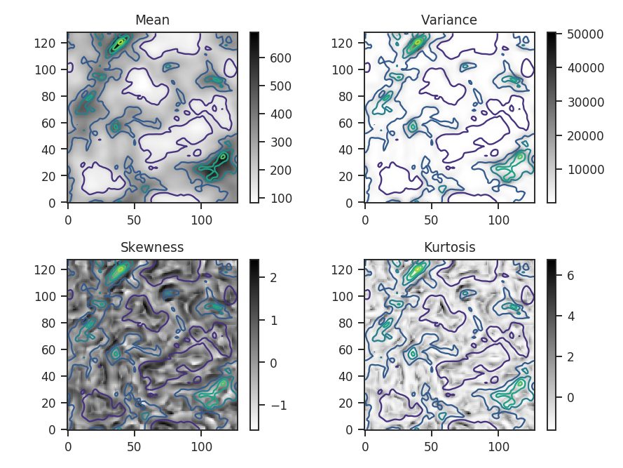
Overlaid on all four plots are the intensity contours from the zeroth moment, making it easier to compare the moment structures to the intensity. Some of the moment maps are more useful than others. For example the mean array is simply a smoothed version of the zeroth moment. The variance map scales closely with the peaks in emission. The skewness and kurtosis maps show perhaps the more interesting products. Both emphasize regions with sharper gradients in the intensity map, and since both are scaled by the variance, they are independent of the intensity scaling.
The moment maps are shown above, but the distributions of the moments are of greater interest for comparing with other data sets. plot_histograms plots, and optionally saves, the histograms:
>>> moments.plot_histograms() # doctest: +SKIP
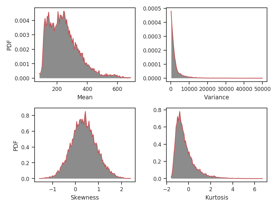
Again, the mean is just a smoothed version of the zeroth moment values. The variance has a strong tail, emphasized by the square term at high intensity peak in the map. The skewness and kurtosis provide distributions of normalized parameters, making it easier to use these quantities for comparing to other data sets.
This example does not include any blanked regions, though observational data often do. To avoid edge effects near these regions, a limit can be set on the minimum fraction of finite points within each region with min_frac. By default, min_frac is set to 0.8. To completely remove edge effects, this parameter can be increased to 1 to reject all regions that contain a NaN. Note that this will increase the size of the blank region by your chosen radius.
Warning
This example uses data that are noiseless. If these data did have noise, it would be critical to remove the noise-dominated regions when computing the skewness and kurtosis, in particular, since they are normalized by the variance. To minimize the effect of noise, the data can be masked beforehand or an array of weights can be passed to down-weight noisy regions. We recommend using the latter method. For example, a weight array could be the inverse squared noise level of the data. Assume the noise level is set to make the signal-to-noise ratio 10 for every pixel in the map:
>>> np.random.seed(3434789)
>>> noise = moment0.data * 0.1 + np.random.normal(0, 0.1, size=moment0.data.shape)  # doctest: +SKIP
>>> moments_weighted = StatMoments(moment0, radius=5 * u.pix,
...                                weights=noise**-2)  # doctest: +SKIP
>>> moments_weighted.run(verbose=True, periodic=True)  # doctest: +SKIP
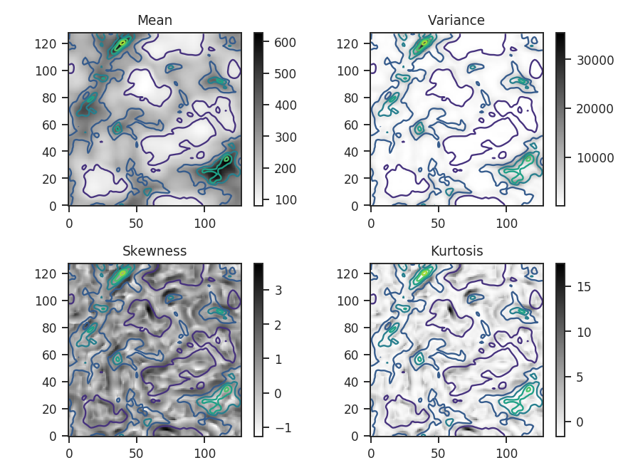
And the associated histograms:
>>> moments_weighted.plot_histograms() # doctest: +SKIP
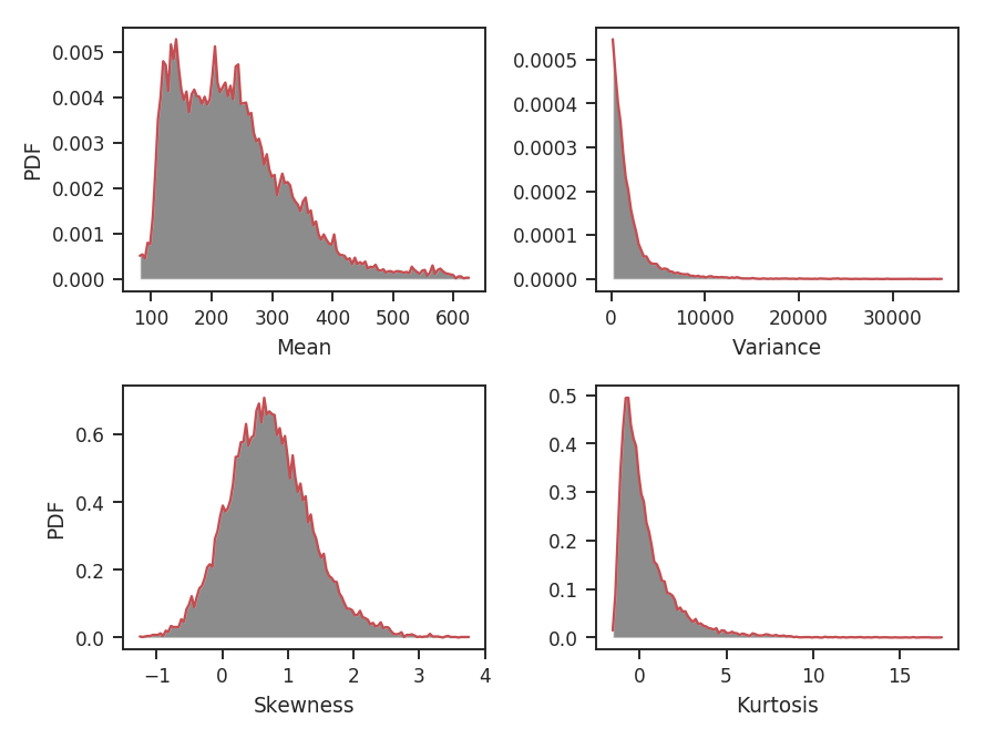
An important consideration when choosing the radius is the balance between tracking small-scale variations and the increased uncertainty when estimating the moments with less data. Burkhart et al. 2010 use approximate formulae for the standard errors of skewness and kurtosis for a normal distribution that are valid for large samples. These are \(\sqrt{6 / n}\) for skewness and \(\sqrt{24 / n}\) for kurtosis, where \(n\) is the number of points. This also assumes all of these points are independent of each other. This typically is not true of observational data, where the data are correlated on at least the beam scale. Each of these points should be considered when choosing the minimum radius appropriate for the data set. For more information on the standard errors, see the sections on skewness and kurtosis on their Wikipedia pages.
What happens if the radius is chosen to be too small, making the higher-order moments highly uncertain? A new radius can be given to run to replace the first one given:
>>> moments.run(verbose=False, radius=2 * u.pix)  # doctest: +SKIP
>>> moments.plot_histograms()  # doctest: +SKIP
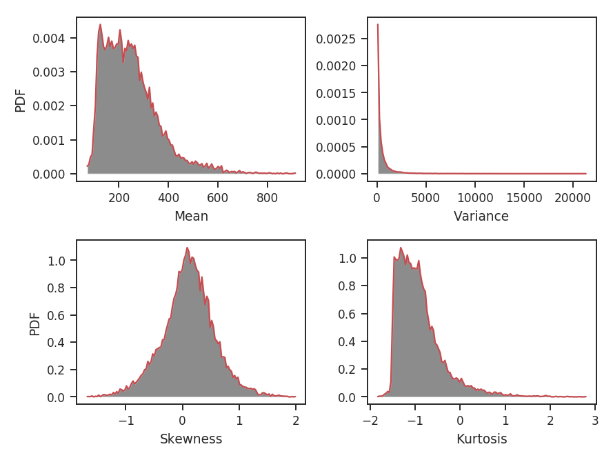
The skewness distribution is narrower, but the kurtosis is wider. The kurtosis uncertainty is larger than the skewness uncertainty, leading to a broader distribution. What are the distribution shapes using larger radii?
>>> moments.run(verbose=False, radius=10 * u.pix)  # doctest: +SKIP
>>> moments.plot_histograms()  # doctest: +SKIP
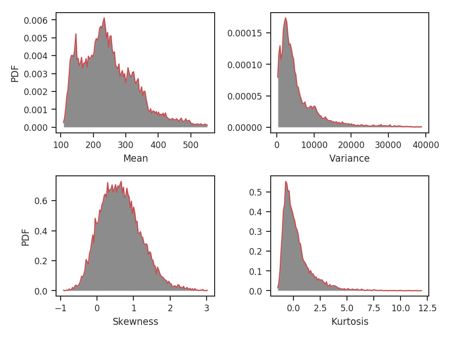
The skewness and kurtosis distributions are not significantly different from the first example, which used radius=5 * u.pix. This seems to suggest that radii in this range give values that are not primarily dominated by the measurement uncertainty. The variance distribution has changed though: its peak is no longer at 0. When averaging over a region larger than the size of most of the structure, the peak of the variance should start to become larger than 0. How about computing moments over a much larger radius?
>>> moments.run(verbose=False, radius=32 * u.pix)  # doctest: +SKIP
>>> moments.plot_histograms()  # doctest: +SKIP
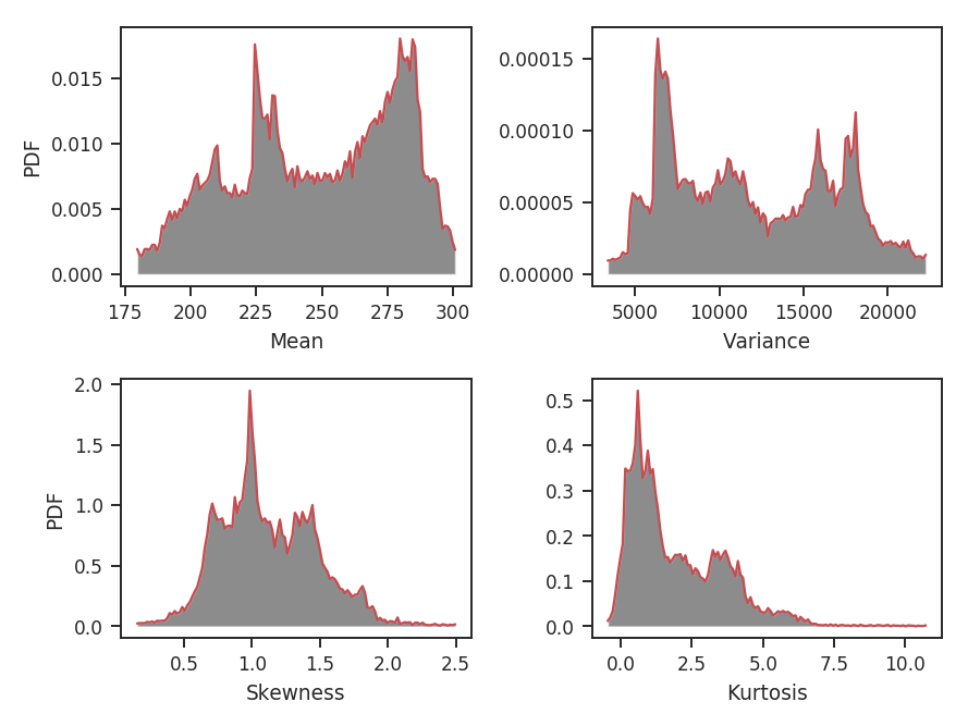
This is clearly too large of a region to be using for this data. A radius of 32 pixels means using a circular region half the size of the image, and there are artifacts dominated by single prominent features in the map, leading to weird multi-model moment distributions.
Because this method relies significantly on the pixel size of the map (for small radii), comparing data sets is best done on a common grid. However, if larger radii are being used, the pixel-to-pixel variation will not be as important.
Often it is more convenient to specify scales in angular or physical units, rather than pixels. radius can be given as either, so long as a distance is provided. For example, assume the distance to the cloud in this data is 250 pc and we want the radius to be 0.23 pc:
>>> moments = StatMoments(moment0, radius=0.23 * u.pc)  # doctest: +SKIP
>>> moments.run(verbose=False, periodic=True)  # doctest: +SKIP
>>> moments.plot_histograms()  # doctest: +SKIP
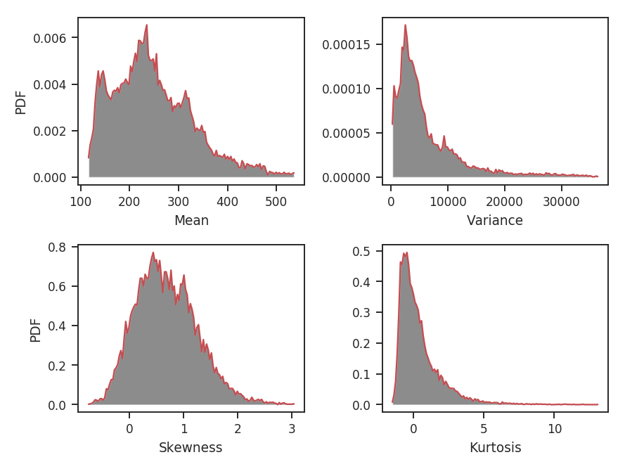
When a radius is given in angular or physical units, the radius of the region used is rounded down to the nearest integer. In this case, 0.23 pc rounds down to 10 pixels and we find the same distributions shown above for the radius=10*u.pix case.
Tsallis Statistics
Overview
The Tsallis statistic was introduced by Tsallis 1988 for describing multi-fractal (non-Gaussian) systems. Its use for describing properties of the ISM has been explored in Esquivel & Lazarian 2010 and Tofflemire et al. 2011. In both of these works, they consider describing an incremental lags in a field by the Tsallis distribution. The specific form of this Tsallis distribution is the q-Gaussian distribution:
where \(a\) is the normalization, \(q\) controls how “peaked” the distribution is (and is therefore closely related to the kurtosis; Moments tutorial), and \(w\) is the width of the distribution. As \(q \rightarrow 1\) the distribution approaches a Gaussian, while \(q > 1\) gives a flattened distribution with heavier tails. The field is a standardized measure of some quantity: \(\Delta f(r) = \left[ f(x, r) - \left< f(x, r) \right>_x \right] / \sqrt{{\rm var}\left[f(x, r)\right]}\), where the angle brackets indicate an average over \(x\). The input quantity is the difference over some scale \(r\) of a field \(f(x)\): \(f(x, r) = f(x) - f(x + r)\). The \(x, r\) are vectors for multi-dimensional data and the formalism is valid for any dimension of data. One distribution is generated for each scale \(r\), and the variation of the distribution parameters with changing \(r\) can be tracked.
Both Esquivel & Lazarian 2010 and Tofflemire et al. 2011 calculate the Tsallis distribution properties for 3D (spatial) and 2D (column density) fields for different sets of simulations. Since TurbuStat is intended to work solely for observable quantities, only the integrated intensity or column density maps can currently be used.
Using
The data in this tutorial are available here.
We need to import the Tsallis code, along with a few other common packages:
>>> from turbustat.statistics import Tsallis
>>> from astropy.io import fits
>>> import astropy.units as u
>>> import numpy as np
And we load in the data:
>>> moment0 = fits.open("Design4_flatrho_0021_00_radmc_moment0.fits")[0] # doctest: +SKIP
With default values, the Tsallis distribution fits are calculated using:
>>> tsallis = Tsallis(moment0).run(verbose=True)  # doctest: +SKIP
lags      logA            w2             q         logA_stderr       w2_stderr         q_stderr      redchisq [1]
pix
---- -------------- -------------- ------------- ---------------- ---------------- ---------------- --------------
 1.0 0.642229857292 0.222031894177 1.72708275041 0.00558780778548 0.00392936618184 0.00103432936045 0.202923321877
 2.0 0.686145334852 0.229079180855 1.71512052919 0.00601337392851 0.00465774887931 0.00120261353862 0.314920328798
 4.0 0.738130813081 0.205824741132 1.74329506331 0.00782571325777 0.00483708991946 0.00165192806993 0.455329606682
 8.0 0.820591668413 0.287364084649 1.70387371009 0.00512574211395 0.00699865080392  0.0016250542739  0.64092221368
16.0  0.83785933956 0.508262278484 1.60949351842 0.00275789013817  0.0115039005934  0.0015760977175 0.613100600322
32.0 0.690126682101 0.852684323374 1.45747128702 0.00207752670078  0.0150332422006 0.00122083964724 0.386135737083
64.0 0.648192026832 0.772095703182 1.43822716004  0.0033147013027  0.0194318148758 0.00200724866629 0.556200738841
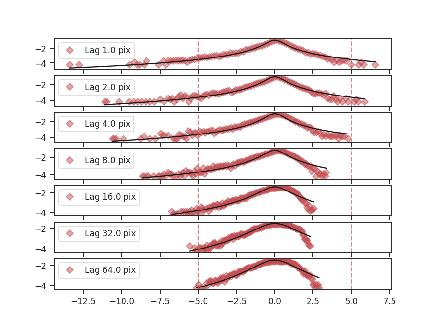
This returns an astropy table of the fits to each of the parameters, their standard errors, and the reduced \(\chi^2\) values (tsallis_table). The figure shows the histograms at each lag and their respective fits. The solid black line is the fit and the dashed red lines indicated which data were used to fit the distribution. The x-axis shows the standardized values of the difference maps at each lag, such that the mean is zero and the standard deviation is one. Because of this, there is no mean parameter fit in the Tsallis distribution. Examining the histograms and the fits is useful for showing where the histograms deviate significantly from the model, something that is difficult to determine from the reduced \(\chi^2\) values alone.
A key to the works of Esquivel & Lazarian 2010 and Tofflemire et al. 2011 is how the fit parameters vary at the different lags. Plots showing the fit parameters as a function of the lag can be shown by running:
>>> tsallis.plot_parameters() # doctest: +SKIP
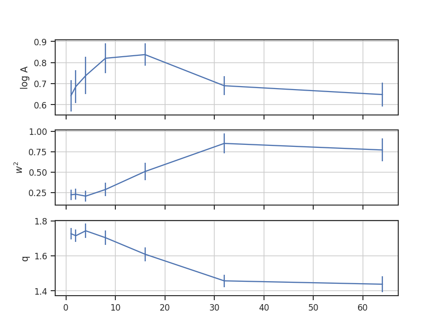
The amplitude of the fit, shown on the top, simply sets the normalization. The more interesting shape parameters \(w^2\) and \(q\) are shown in the second and third panels. As explained in the overview, \(w^2\) is analogous to the width of a Gaussian curve, while \(q\) determines how peaked the distribution is and if closely related to the kurtosis.
Warning
These parameters are not independent in this fit! The plot shows that the two are anti-correlated. This means that their standard errors are underestimated, even if the requirements for the non-linear least squares fit are met by the data. When examining and interpreting the parameter fits, this covariance should be kept in mind.
The lag values were automatically determined in the previous example. The default lag size, when none are provided, is to use powers of two up to half of the smallest axis size in the image. The example data is a 128-by-128 pixel image and so the lags used are 1, 2, 4, 8, 16, 32, and 64 pixels. If custom values for the lags are given, they must have an attached unit in pixel, angular or physical units. The latter requires passing a distance to Tsallis. For example, assume that the region in the simulated data is located at a distance of 250 pc:
>>> distance = 250 * u.pc
>>> phys_lags = np.arange(0.025, 0.5, 0.05) * u.pc
>>> tsallis = Tsallis(moment0, lags=phys_lags, distance=distance)  # doctest: +SKIP
>>> tsallis.run(verbose=True)  # doctest: +SKIP
 lags      logA            w2             q         logA_stderr       w2_stderr          q_stderr      redchisq [1]
  pc
----- -------------- -------------- ------------- ---------------- ---------------- ----------------- --------------
0.025 0.642229857292 0.222031894177 1.72708275041 0.00558780778548 0.00392936618184  0.00103432936045 0.202923321877
0.075 0.705449362909 0.218319248608 1.72354565147 0.00737330905613 0.00519808619425  0.00152701310901 0.412646518168
0.125 0.789721056553 0.229683344052 1.75057343162 0.00538732578554 0.00423363268573  0.00128094113344 0.409462321776
0.175 0.812924754652  0.26193847697 1.72229438044 0.00582788661761 0.00641904864759   0.0016875791307 0.591453809951
0.225 0.819013579917 0.327952306938 1.68254342712 0.00414539826435 0.00769391172561  0.00152138140139 0.602749326188
0.275  0.84019947484  0.43700081371 1.65129052189 0.00319162263733    0.01060267014  0.00161948565142 0.572638168121
0.325 0.775203769634 0.638231616687 1.55766127541 0.00157464300665  0.0112005405935 0.000945367175158 0.390439429254
0.375  0.83785933956 0.508262278484 1.60949351842 0.00275789013817  0.0115039005934   0.0015760977175 0.613100600322
0.425  0.82517267059 0.439101136039 1.61618300379 0.00412874845191  0.0131188204054  0.00230155968913 0.823108982477
0.475 0.780592562471 0.538751135268 1.56786712441 0.00244860804161  0.0114898743283  0.00145531646909 0.571370986301
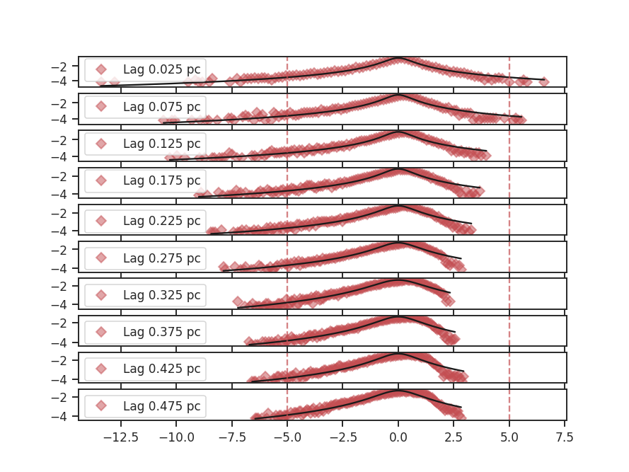
The lags given here correspond to pixel scales of 1 to about 21 pixels. Whenever lags are given that convert to a fraction of a pixel, the next smallest integer value is used as the lag. The lags given in the output table are always kept in the units they were given in, not the equivalent pixel size in the image.
Calculating the difference in the image at a given lag requires shuffling the data in different directions, and then taking its difference (similar to the SCF). If the data is periodic in the spatial dimensions, like the example data used here, we want to keep the portion of the data that was rolled passed the edge. The periodic boundary handling is enabled by default. To disable treating the edges as periodic, periodic=False can be passed:
>>> tsallis_noper = Tsallis(moment0).run(verbose=True, periodic=False)  # doctest: +SKIP
lags      logA             w2             q         logA_stderr       w2_stderr         q_stderr      redchisq [1]
pix
---- -------------- --------------- ------------- ---------------- ---------------- ---------------- --------------
 1.0 0.897012384613 0.0118349188867 2.23324265255   0.166620498872 0.00017563398593 0.00483817878284  1.05048714536
 2.0 0.896022807195  0.163157700047 1.82635786848  0.0143795839865 0.00540543040786 0.00328264939428 0.856843401609
 4.0 0.786658543433  0.300038576861 1.68212189627 0.00663851190583  0.0102461537338 0.00237396765607 0.760443068549
 8.0 0.783914175933  0.357145631871 1.65368430773  0.0046022510611  0.0103614381214 0.00184930165344 0.667505258089
16.0 0.790689760595  0.674952448852   1.546507737 0.00215124566812  0.0142829674771 0.00129998567864 0.557924881035
32.0 0.713731153997  0.771328751704 1.47897488745 0.00283752579166  0.0172594116452 0.00169658285939 0.475827962986
64.0 0.783452488524  0.742301900184 1.52244838954 0.00300307934231  0.0179167808952 0.00177362923754 0.606593199807
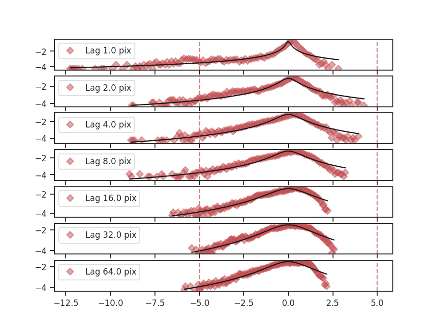
The histograms are quite different, partially because we are throwing out extra data as the lags increase.
Throughout these examples, the fitting has been limited to \(\pm 5\) of the standard deviation, as indicated by the dashed red lines in the histogram plots. If the limits need to be changed, the sigma_clip keyword can be passed:
>>> tsallis = Tsallis(moment0).run(verbose=True, sigma_clip=3)  # doctest: +SKIP
lags      logA            w2             q         logA_stderr       w2_stderr         q_stderr       redchisq [1]
pix
---- -------------- -------------- ------------- ---------------- ---------------- ---------------- ---------------
 1.0 0.676668795627  0.29391426291 1.71669037083 0.00157383166087 0.00261634517218 0.00198839049982  0.057608469887
 2.0 0.745791738309 0.322366742708 1.72147347306 0.00183938037718 0.00274517409678 0.00215767963285 0.0624568707002
 4.0 0.673011928843 0.444372636313 1.60204004903 0.00201910360961 0.00408585675961 0.00216448599475 0.0701353589419
 8.0 0.726710296991 0.555894748784 1.57342987012 0.00563401682478 0.00969116551888 0.00448516671654  0.127621910509
16.0 0.789370379072 0.767631108873 1.55063965451  0.0107467878091  0.0179646081854 0.00625731804422  0.166963375365
32.0 0.718628894604  1.08365218957 1.46486083229 0.00825834877876  0.0154641791221  0.0038873537526 0.0866162406828
64.0 0.502202769666  1.19658833745 1.32473447015 0.00947708275941  0.0217408584935 0.00436354465126  0.120069117864
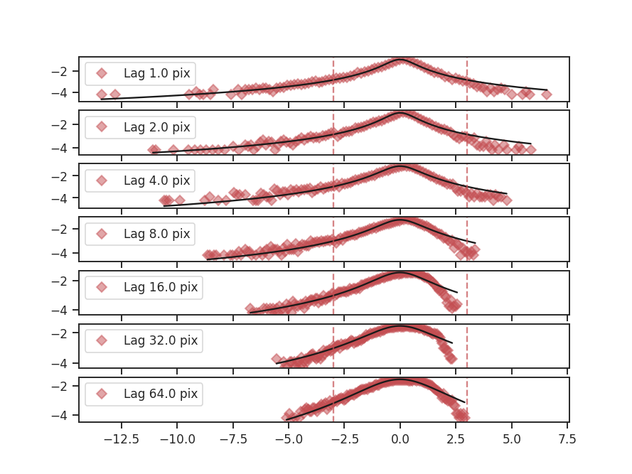
Since there are still many points to fit, the fit qualities have not significantly worsened from lowering the sigma limit. However the fit parameters have changed:
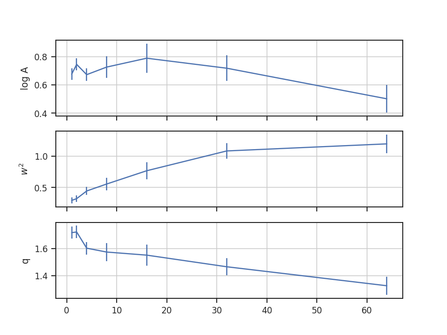
The same basic trend of the fit parameters with increasing lag size can be seen, but the values have changed by a large amount. This is another example that caution needs to be used when interpreting the fit standard errors and the reduced \(\chi^2\).
One final parameter can be changed: the number of bins used to create the histogram. For most images, the number of data points will be large, and so the default bin number is set to be the square-root of the number of data points. This is a good estimate in the limit of many data points, but will become poor if there are less than \(\sim100\) data points from the image. To change the number of bins used, num_bins can be passed to run.
Velocity Channel Analysis (VCA)
Overview
A major advantage of a spectral-line data cube, rather than an integrated two-dimensional image, is that it captures aspects of both the density and velocity fluctuations in the field of observation. Lazarian & Pogosyan 2000 and Lazarian & Pogosyan 2004 derived how the power spectrum from a cube depends on the statistics of the density and velocity fields for the 21-cm Hydrogen line, allowing for each of their properties to be examined (provided the data have sufficient spectral resolution).
The Lazarian & Pogosyan theory predicts two regimes based on the the power-spectrum slope: the shallow (\(n < -3\)) and the steep (\(n < -3\)) regimes. In the case of optically thick line emission, Lazarian & Pogosyan 2004 show that the slope saturates to \(n = -3\) (see Burkhart et al. 2013 as well). The VCA predictions in these different regimes are shown in Table 1 of Chepurnov & Lazarian 2009 (also see Table 3 in Lazarian 2009). The complementary Velocity Coordinate Spectrum can be used in tandem with VCA.
Using
The data in this tutorial are available here.
We need to import the VCA class, along with a few other common packages:
>>> from turbustat.statistics import VCA
>>> from astropy.io import fits
And we load in the data cube:
>>> cube = fits.open("Design4_flatrho_0021_00_radmc.fits")[0] # doctest: +SKIP
The VCA spectrum is computed using:
>>> vca = VCA(cube)  # doctest: +SKIP
>>> vca.run(verbose=True)  # doctest: +SKIP
                            OLS Regression Results
==============================================================================
Dep. Variable:                      y   R-squared:                       0.973
Model:                            OLS   Adj. R-squared:                  0.973
Method:                 Least Squares   F-statistic:                     3188.
Date:                Thu, 20 Jul 2017   Prob (F-statistic):           1.75e-71
Time:                        15:14:32   Log-Likelihood:                -1.2719
No. Observations:                  91   AIC:                             6.544
Df Residuals:                      89   BIC:                             11.57
Df Model:                           1
Covariance Type:            nonrobust
==============================================================================
                 coef    std err          t      P>|t|      [0.025      0.975]
------------------------------------------------------------------------------
const          2.3928      0.058     41.036      0.000       2.277       2.509
x1            -4.2546      0.075    -56.459      0.000      -4.404      -4.105
==============================================================================
Omnibus:                        4.747   Durbin-Watson:                   0.069
Prob(Omnibus):                  0.093   Jarque-Bera (JB):                4.622
Skew:                          -0.550   Prob(JB):                       0.0992
Kurtosis:                       2.916   Cond. No.                         4.40
==============================================================================
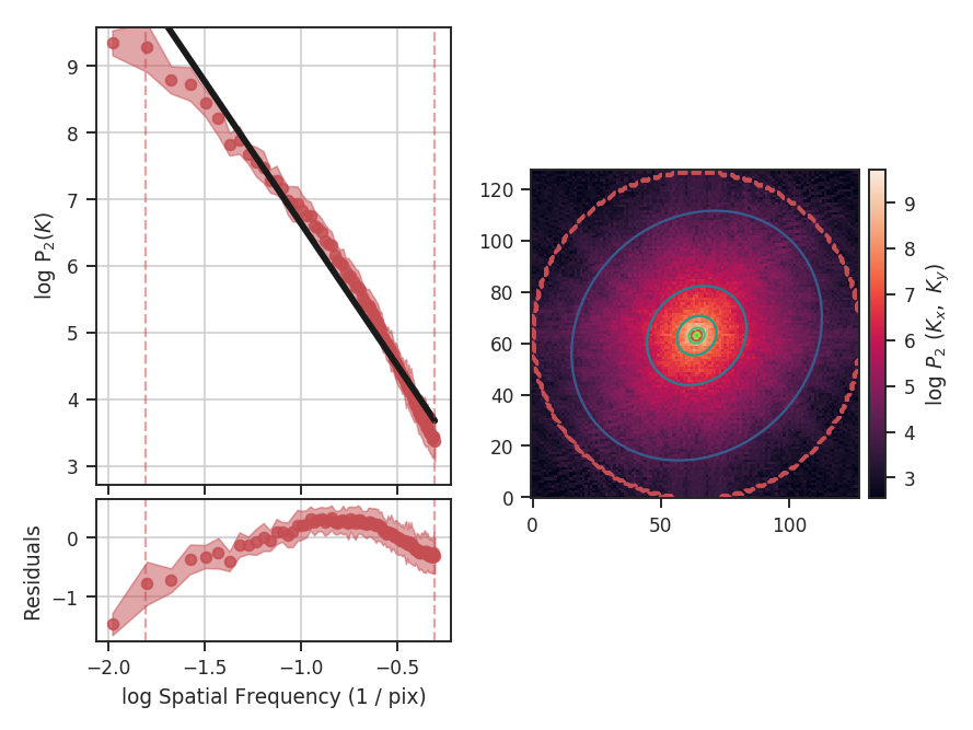
The code returns a summary of the one-dimensional fit and a figure showing the one-dimensional spectrum and model on the left, and the two-dimensional power-spectrum on the right. If fit_2D=True is set in run (the default setting), the contours on the two-dimensional power-spectrum are the fit using an elliptical power-law model. We will discuss the models in more detail below. The dashed red lines (or contours) on both plots are the limits of the data used in the fits. See the PowerSpectrum tutorial for a discussion of the two-dimensional fitting.
The VCA power spectrum from this simulated data cube is \(-4.25\pm0.08\), which is steeper than the power spectrum we found using the zeroth moment (PowerSpectrum tutorial). However, as was the case for the power-spectrum of the zeroth moment, there are deviations from a single power-law on small scales due to the inertial range in the simulation. The spatial frequencies used in the fit can be limited by setting low_cut and high_cut. The inputs should have frequency units in pixels, angle, or physical units. In this case, we will limit the fitting between frequencies of 0.02 / pix and 0.1 / pix (where the conversion to pixel scales in the simulation is just 1 / freq):
>>> vca.run(verbose=True, xunit=u.pix**-1, low_cut=0.02 / u.pix,
...         high_cut=0.1 / u.pix)  # doctest: +SKIP
                            OLS Regression Results
==============================================================================
Dep. Variable:                      y   R-squared:                       0.985
Model:                            OLS   Adj. R-squared:                  0.984
Method:                 Least Squares   F-statistic:                     866.6
Date:                Thu, 20 Jul 2017   Prob (F-statistic):           2.77e-13
Time:                        15:28:29   Log-Likelihood:                 17.850
No. Observations:                  15   AIC:                            -31.70
Df Residuals:                      13   BIC:                            -30.28
Df Model:                           1
Covariance Type:            nonrobust
==============================================================================
                 coef    std err          t      P>|t|      [0.025      0.975]
------------------------------------------------------------------------------
const          3.7695      0.134     28.031      0.000       3.479       4.060
x1            -3.0768      0.105    -29.438      0.000      -3.303      -2.851
==============================================================================
Omnibus:                        1.873   Durbin-Watson:                   2.409
Prob(Omnibus):                  0.392   Jarque-Bera (JB):                1.252
Skew:                          -0.684   Prob(JB):                        0.535
Kurtosis:                       2.641   Cond. No.                         13.5
==============================================================================
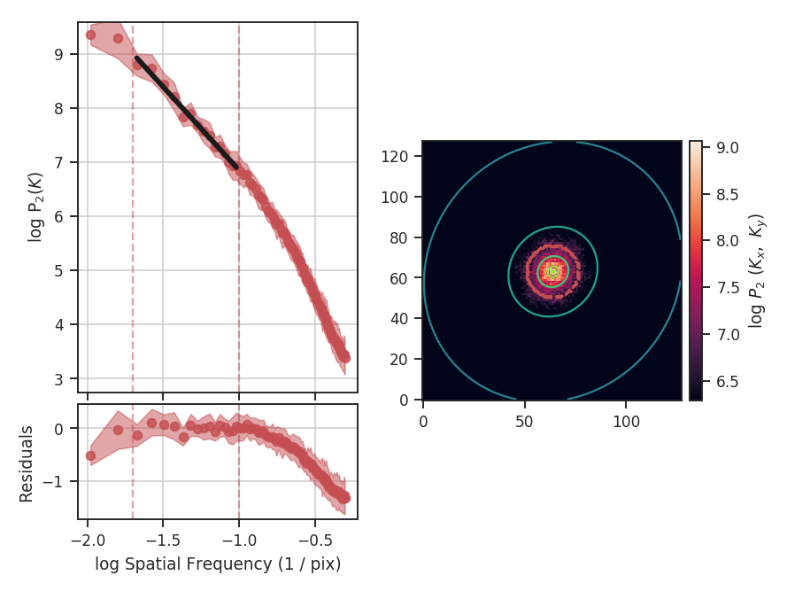
With the fit limited to the valid region, we find a shallower slope of \(-3.1\pm0.1\) and a better fit to the model. low_cut and high_cut can also be given as spatial frequencies in angular units (e.g., u.deg**-1). When a distance is given, the low_cut and high_cut can also be given in physical frequency units (e.g., u.pc**-1).
This example has used the default ordinary least-squares fitting. A weighted least-squares can be enabled with weighted_fit=True (this cannot be used for the segmented model described below).
Breaks in the power-law behaviour in observations (and higher-resolution simulations) can result from differences in the physical processes dominating at those scales. To capture this behaviour, VCA can be passed a break point to enable fitting with a segmented linear model (Lm_Seg; see the description given in the PowerSpectrum tutorial). The 2D fitting is disabled for this section as it does handle fitting break points. In this example, we will assume a distance of 250 pc in order to show the power spectrum in physical units:
>>> vca = VCA(cube, distance=250 * u.pc)  # doctest: +SKIP
>>> vca.run(verbose=True, xunit=u.pc**-1, low_cut=0.02 / u.pix,
...         high_cut=0.4 / u.pix, fit_kwargs=dict(brk=0.1 / u.pix),
...         fit_2D=False)  # doctest: +SKIP
                            OLS Regression Results
==============================================================================
Dep. Variable:                      y   R-squared:                       0.998
Model:                            OLS   Adj. R-squared:                  0.998
Method:                 Least Squares   F-statistic:                 1.113e+04
Date:                Thu, 20 Jul 2017   Prob (F-statistic):           2.66e-90
Time:                        16:19:33   Log-Likelihood:                 101.91
No. Observations:                  71   AIC:                            -195.8
Df Residuals:                      67   BIC:                            -186.8
Df Model:                           3
Covariance Type:            nonrobust
==============================================================================
                 coef    std err          t      P>|t|      [0.025      0.975]
------------------------------------------------------------------------------
const          3.6333      0.053     68.784      0.000       3.528       3.739
x1            -3.1814      0.047    -67.916      0.000      -3.275      -3.088
x2            -2.4558      0.094    -26.152      0.000      -2.643      -2.268
x3            -0.0097      0.027     -0.355      0.724      -0.065       0.045
==============================================================================
Omnibus:                        8.205   Durbin-Watson:                   1.148
Prob(Omnibus):                  0.017   Jarque-Bera (JB):                7.707
Skew:                          -0.772   Prob(JB):                       0.0212
Kurtosis:                       3.469   Cond. No.                         20.8
==============================================================================
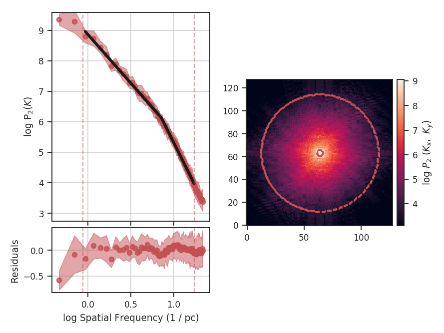
By incorporating the break, we find a better quality fit to this portion of the power-spectrum. We also find that the slope before the break (i.e., in the inertial range), the slope is consistent with the slope from the zeroth moment (PowerSpectrum tutorial). The break point was moved significantly from the initial guess, which we had set to the upper limit of the inertial range:
>>> vca.brk  # doctest: +SKIP
<Quantity 0.1624771454997838 1 / pix>
>>> vca.brk_err  # doctest: +SKIP
<Quantity 0.010241094948585336 1 / pix>
From the figure, this is where the curve deviates from the power-law on small scales. With our assigned distance, the break point corresponds to a physical scale of:
>>> vca._physical_size / vca.brk.value  # doctest: +SKIP
<Quantity 0.14082499334584425 pc>
vca._physical_size is the spatial size of one pixel (assuming the spatial dimensions have square pixels in the celestial frame).
The values of the slope after the break point (x2) in the fit description is defined relative to the first slope. Its actual slope would then be the sum of x1 and x2. The slopes and their uncertainties can be accessed through:
>>> vca.slope  # doctest: +SKIP
array([-3.18143757, -5.63724147])
>>> vca.slope_err  # doctest: +SKIP
array([ 0.04684344,  0.104939  ])
The slope above the break point is within the uncertainty of the slope we found in the second example (\(-3.1\pm0.1\)). The uncertainty we find here is nearly half of the previous one since more points have been used in this fit.
The Lazarian & Pogosyan theory predicts that the VCA power-spectrum depends on the size of the velocity slices in the data cube (e.g., Stanimirovic & Lazarian 2001). VCA allows for the velocity channel thickness to be changed with channel_width. This runs a routine that down-samples the spectral dimension to match the given channel width. We can re-run VCA on this data with a channel width of \(\sim 400\) m / s, and compare to the original slope:
>>> vca_thicker_channel = VCA(cube, distance=250 * u.pc,
...                           channel_width=400 * u.m / u.s,
...                           downsample_kwargs=dict(method='downsample'))  # doctest: +SKIP
>>> vca_thicker.run(verbose=True, xunit=u.pc**-1, low_cut=0.02 / u.pix,
...                 high_cut=0.4 / u.pix,
...                 fit_kwargs=dict(brk=0.1 / u.pix), fit_2D=False)  # doctest: +SKIP
                       OLS Regression Results
==============================================================================
Dep. Variable:                      y   R-squared:                       0.998
Model:                            OLS   Adj. R-squared:                  0.998
Method:                 Least Squares   F-statistic:                     9739.
Date:                Thu, 20 Jul 2017   Prob (F-statistic):           2.29e-88
Time:                        19:00:25   Log-Likelihood:                 94.310
No. Observations:                  71   AIC:                            -180.6
Df Residuals:                      67   BIC:                            -171.6
Df Model:                           3
Covariance Type:            nonrobust
==============================================================================
                 coef    std err          t      P>|t|      [0.025      0.975]
------------------------------------------------------------------------------
const          1.4422      0.057     25.516      0.000       1.329       1.555
x1            -3.2388      0.051    -64.014      0.000      -3.340      -3.138
x2            -2.8668      0.108    -26.651      0.000      -3.081      -2.652
x3             0.0116      0.030      0.385      0.702      -0.049       0.072
==============================================================================
Omnibus:                        7.262   Durbin-Watson:                   1.043
Prob(Omnibus):                  0.026   Jarque-Bera (JB):                6.646
Skew:                          -0.720   Prob(JB):                       0.0361
Kurtosis:                       3.418   Cond. No.                         20.9
==============================================================================

With the original spectral resolution, the slope in the inertial range was already consistent with the “thickest slice” case, the zeroth moment. The slope here remains consistent with the zeroth moment power-spectrum, so for this data set of \(^{13}{\rm CO}\), there is no evolution in the spectrum with channel size.
An alternative method to change the channel width can be used by specifying downsample_kwargs=dict(method='regrid'). The spectral axis of the cube is smoothed with a Gaussian kernel and down-sampled by interpolating to a new spectral axis with width channel_width (see the spectral-cube documentation).
Constraints on the azimuthal angles used to compute the one-dimensional power-spectrum can also be given:
>>> vca = VCA(cube)  # doctest: +SKIP
>>> vca.run(verbose=True, xunit=u.pix**-1, low_cut=0.02 / u.pix,
...         high_cut=0.1 / u.pix,
...         radial_pspec_kwargs={"theta_0": 1.13 * u.rad, "delta_theta": 40 * u.deg})  # doctest: +SKIP
                            OLS Regression Results
==============================================================================
Dep. Variable:                      y   R-squared:                       0.958
Model:                            OLS   Adj. R-squared:                  0.955
Method:                 Least Squares   F-statistic:                     298.9
Date:                Fri, 29 Sep 2017   Prob (F-statistic):           2.36e-10
Time:                        14:57:53   Log-Likelihood:                 11.566
No. Observations:                  15   AIC:                            -19.13
Df Residuals:                      13   BIC:                            -17.71
Df Model:                           1
Covariance Type:            nonrobust
==============================================================================
                 coef    std err          t      P>|t|      [0.025      0.975]
------------------------------------------------------------------------------
const          4.2111      0.204     20.597      0.000       3.769       4.653
x1            -2.7475      0.159    -17.290      0.000      -3.091      -2.404
==============================================================================
Omnibus:                       18.967   Durbin-Watson:                   2.608
Prob(Omnibus):                  0.000   Jarque-Bera (JB):               18.398
Skew:                          -1.869   Prob(JB):                     0.000101
Kurtosis:                       6.932   Cond. No.                         13.5
==============================================================================
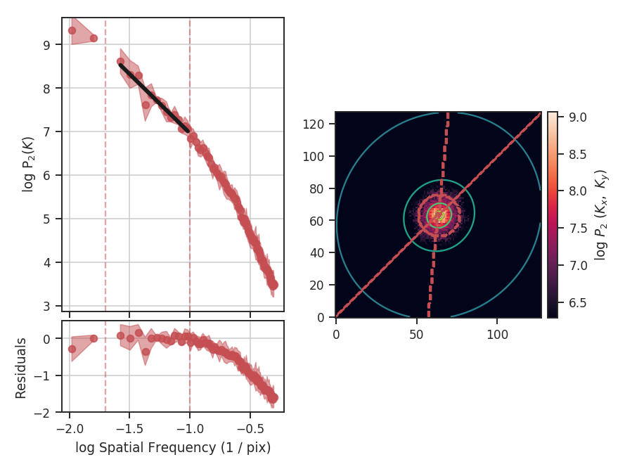
The azimuthal limits now appear as contours on the two-dimensional power-spectrum in the figure. See the PowerSpectrum tutorial for more information on giving azimuthal constraints.
If strong emission continues to the edge of the map (and the map does not have periodic boundaries), ringing in the FFT can introduce a cross pattern in the 2D power-spectrum. This effect and the use of apodizing kernels to taper the data is covered here.
Most observational data will be smoothed over the beam size, which will steepen the power spectrum on small scales. To account for this, the 2D power spectrum can be divided by the beam response. This is demonstrated here for spatial power-spectra.
Velocity Coordinate Spectrum (VCS)
Overview
The Velocity Coordinate Spectrum (VCS) was present in the theoretical framework of Lazarian & Pogosyan 2000, and further developed in Lazarian & Pogosyan 2006. The VCS is complementary to the VCA, but rather than integrating over the spectral dimension in the VCA, the spatial dimensions are integrated over. This results in a 1D power-spectrum whose properties and shape are set by the underlying turbulent velocity and density fields, and the typical velocity dispersion and beam size of the data.
There are two asymptotic regimes of the VCS corresponding to high and low resolution (Lazarian & Pogosyan 2006). The transition between these regimes depends on the spatial resolution (i.e., beam size) of the data, the spectral resolution of the data, and the velocity dispersion. The current VCS implementation in TurbuStat fits a broken linear model to approximate the asymptotic regimes, rather than fitting with the full VCS formalism (Chepurnov et al. 2010, Chepurnov et al. 2015). We assume that the break point lies at the transition point between the regimes and label velocity frequencies smaller than the break as “large-scale” and frequencies larger than the break as “small-scale”.
A summary of the VCS asymptotic regimes is given in Table 3 of Lazarian 2009.
Using
The data in this tutorial are available here.
We need to import the VCS class, along with a few other common packages:
>>> from turbustat.statistics import VCS
>>> from astropy.io import fits
And we load in the data cube:
>>> cube = fits.open("Design4_flatrho_0021_00_radmc.fits")[0] # doctest: +SKIP
The VCA spectrum is computed using:
>>> vcs = VCS(cube)  # doctest: +SKIP
>>> vcs.run(verbose=True)  # doctest: +SKIP
                            OLS Regression Results
==============================================================================
Dep. Variable:                      y   R-squared:                       0.909
Model:                            OLS   Adj. R-squared:                  0.908
Method:                 Least Squares   F-statistic:                     815.9
Date:                Fri, 21 Jul 2017   Prob (F-statistic):          3.55e-127
Time:                        16:18:42   Log-Likelihood:                -402.80
No. Observations:                 249   AIC:                             813.6
Df Residuals:                     245   BIC:                             827.7
Df Model:                           3
Covariance Type:            nonrobust
==============================================================================
                 coef    std err          t      P>|t|      [0.025      0.975]
------------------------------------------------------------------------------
const        -11.4835      0.231    -49.755      0.000     -11.938     -11.029
x1            -9.7426      0.232    -41.915      0.000     -10.200      -9.285
x2             7.4106      2.683      2.762      0.006       2.126      12.696
x3            -0.0399      0.314     -0.127      0.899      -0.658       0.578
==============================================================================
Omnibus:                      133.751   Durbin-Watson:                   0.042
Prob(Omnibus):                  0.000   Jarque-Bera (JB):             1872.647
Skew:                          -1.766   Prob(JB):                         0.00
Kurtosis:                      15.962   Cond. No.                         44.9
==============================================================================
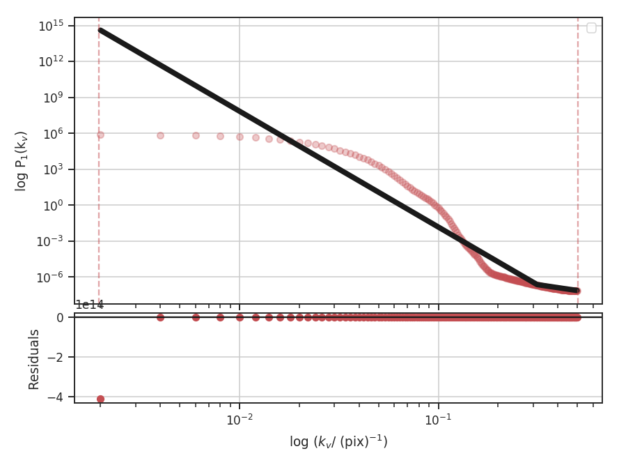
By default, the VCS spectrum will be fit to a segmented linear model with one break point (see the Power Spectrum tutorial for a more detailed explanation of the model). If no break points are specified, a spline is used to estimate the location of break points, each of which are tried until a valid fit is found.
With the default settings, the fit is horrendous. This is due to the model’s current limitation of fitting with a single break point. For these simulated data, there is no information on spectral frequencies below the thermal line width. This cube was created from an isothermal simulation, and at a temperature of 10 K, the thermal line width of \(\sim 200\) m / s is oversampled by the 40 m /s channels. We can avoid fitting this region by setting frequency constraints:
>>> vcs.run(verbose=True, high_cut=0.17 / u.pix)  # doctest: +SKIP
                            OLS Regression Results
==============================================================================
Dep. Variable:                      y   R-squared:                       0.988
Model:                            OLS   Adj. R-squared:                  0.987
Method:                 Least Squares   F-statistic:                     2140.
Date:                Fri, 21 Jul 2017   Prob (F-statistic):           2.90e-76
Time:                        16:29:33   Log-Likelihood:                -37.805
No. Observations:                  84   AIC:                             83.61
Df Residuals:                      80   BIC:                             93.33
Df Model:                           3
Covariance Type:            nonrobust
==============================================================================
                 coef    std err          t      P>|t|      [0.025      0.975]
------------------------------------------------------------------------------
const          1.8245      0.379      4.819      0.000       1.071       2.578
x1            -1.8412      0.219     -8.404      0.000      -2.277      -1.405
x2           -14.8271      0.412    -35.968      0.000     -15.648     -14.007
x3             0.1035      0.167      0.621      0.536      -0.228       0.435
==============================================================================
Omnibus:                       10.043   Durbin-Watson:                   0.058
Prob(Omnibus):                  0.007   Jarque-Bera (JB):                3.501
Skew:                          -0.116   Prob(JB):                        0.174
Kurtosis:                       2.027   Cond. No.                         21.4
==============================================================================
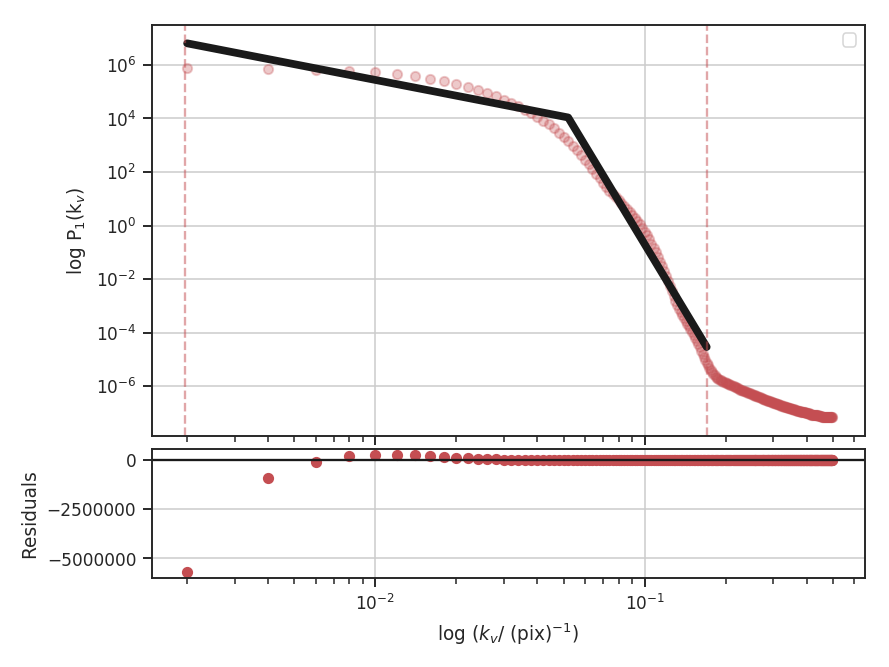
high_cut is set to ignore scales below \(\sim 240\) m / s, just slightly larger than the thermal line width. To see this more clearly, we can create the same plot above in velocity units:
>>> vcs.run(verbose=True, high_cut=0.17 / u.pix,
...         xunit=(u.m / u.s)**-1)  # doctest: +SKIP
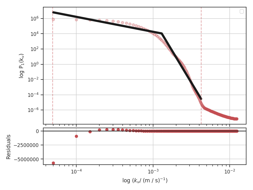
The dotted lines, indicating the fitting extents, are now more easily understood. The lower limit, at about \(4 \times 10^{-3} {\rm m / s}^{-1}\) corresponds to \(1 / \left(4 \times 10^{-3}\right) = 250 {\rm m / s}\).
This is still not an optimal fit. There are large deviations as the single break-point model tries to interpret the smooth transition at large scales. This flattening at large scales could be from the periodic box condition in the simulation: there is effectively a maximum size cut-off at the box size beyond which there is no additional energy. For the next example, assume that this is indeed the case and that we can remove this region from the fit:
>>> vcs.run(verbose=True, high_cut=0.17 / u.pix, low_cut=6e-4 / (u.m / u.s),
...         xunit=(u.m / u.s)**-1)   # doctest: +SKIP
                            OLS Regression Results
==============================================================================
Dep. Variable:                      y   R-squared:                       0.996
Model:                            OLS   Adj. R-squared:                  0.996
Method:                 Least Squares   F-statistic:                     5443.
Date:                Fri, 21 Jul 2017   Prob (F-statistic):           6.70e-81
Time:                        17:10:57   Log-Likelihood:                 15.889
No. Observations:                  72   AIC:                            -23.78
Df Residuals:                      68   BIC:                            -14.67
Df Model:                           3
Covariance Type:            nonrobust
==============================================================================
                 coef    std err          t      P>|t|      [0.025      0.975]
------------------------------------------------------------------------------
const         -8.8409      0.275    -32.183      0.000      -9.389      -8.293
x1            -9.1948      0.217    -42.371      0.000      -9.628      -8.762
x2           -12.3859      0.488    -25.404      0.000     -13.359     -11.413
x3            -0.0062      0.093     -0.067      0.947      -0.191       0.179
==============================================================================
Omnibus:                        6.011   Durbin-Watson:                   0.067
Prob(Omnibus):                  0.050   Jarque-Bera (JB):                5.617
Skew:                          -0.476   Prob(JB):                       0.0603
Kurtosis:                       3.983   Cond. No.                         34.7
==============================================================================
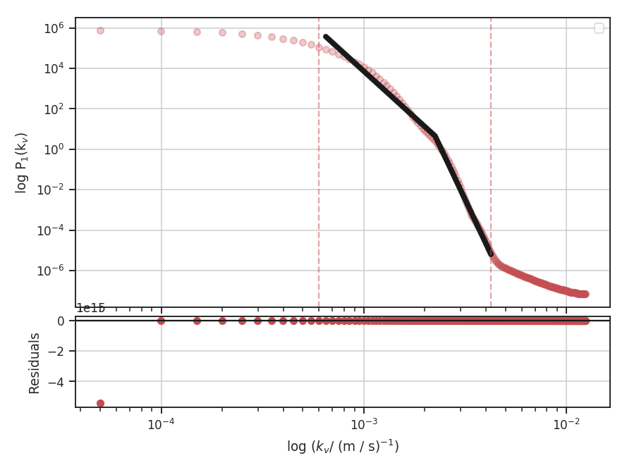
This appears to be a better fit! Also, note that the low_cut and high_cut parameters can be given in pixel or spectral frequency units. We estimated low_cut from the previous example, where the plot was already in spectral frequency units.
Based on the power spectrum slope of \(-3.2\pm0.1\) we found using the zeroth moment map (Power Spectrum tutorial), this data is in the steep regime, where density fluctuations do not dominate at any spectral scale. Using the asymptotic case from Fig. 2 in Lazarian & Pogosyan 2006, the slopes should be close to \(-6 / m\) at small scales and \(-2 / m\) on large scales, where \(m\) is the index of the velocity field. The second slope in the fit summary (x2) is defined relative to the first slope (x1). The true slopes can be accessed through:
>>> vcs.slope  # doctest: +SKIP
array([ -9.19479557, -21.58069847])
>>> vcs.slope_err  # doctest: +SKIP
array([ 0.21700618,  0.53366172])
Since, in this regime, both components only rely on the velocity field, they should both give a consistent estimate of \(m\):
>>> -2 / vcs.slope[0]  # doctest: +SKIP
0.21751435186363388
>>> - 6 / vcs.slope[1]  # doctest: +SKIP
0.2780262190776282
Each component does give a similar estimate for \(m\). There is the additional issue with the simulated data as to how the inertial range should be handled. Certainly the slope at smaller scales is made steeper if portions are outside the spatial inertial range.
While we find a good fit to the data, the VCS transition between the two regimes is smoothed over. This is a break down of assuming the asymptotic regimes, and is a break down of the simplified segmented linear model that has been used. The model presented in Chepurnov et al. 2010 and Chepurnov et al. 2015, which account for a smooth transition over the entire spectrum, will be a more effective and useful choice. This model will be included in a future release of TurbuStat.
Wavelets
Overview
A wavelet transform can be used to filter structure on certain scales, where the scale is typically related to the size and choice of wavelet kernel. By calculating the amount of structure using different sized kernels, the amount of structure on different scales can be calculated. This makes the technique similar to the power-spectrum, but the power at given scale is calculated in the image domain. This approach was introduced for use on astrophysical turbulence by Gill & Henriksen 1990. They used a Mexican-Hat (or Ricker) wavelet for the transform and used the sum of positive values in each filtered map to produce a one-dimensional spectrum between the scale and amount of structure at that scale.
This technique has many similarities to Delta-Variance (see comparison in Zielinsky & Stutzki 1999). Both create a set of filtered maps at different wavelet scales, though the Delta-Variance splits the wavelet kernel into separate component and normalizes by a weight map to reduce edge effects. From the filtered maps, the Delta-Variance measures the variance across the entire map to estimate the amount of structure, while the Wavelet transform assumes the amount of structure is represented by the total of the positive values. From both methods, the slope of the one-dimensional spectrum is the desired measurement.
Using
The data in this tutorial are available here.
We need to import the Wavelet class, along with a few other common packages:
>>> import numpy as np
>>> from turbustat.statistics import Wavelet
>>> from astropy.io import fits
>>> import astropy.units as u
And we load in the data:
>>> moment0 = fits.open("Design4_flatrho_0021_00_radmc_moment0.fits")[0] # doctest: +SKIP
The default wavelet transform of the zeroth moment is calculated as:
>>> wavelet = Wavelet(moment0).run(verbose=True)  # doctest: +SKIP
                            OLS Regression Results
==============================================================================
Dep. Variable:                      y   R-squared:                       0.954
Model:                            OLS   Adj. R-squared:                  0.953
Method:                 Least Squares   F-statistic:                     1001.
Date:                Tue, 01 Aug 2017   Prob (F-statistic):           8.36e-34
Time:                        18:07:44   Log-Likelihood:                 97.550
No. Observations:                  50   AIC:                            -191.1
Df Residuals:                      48   BIC:                            -187.3
Df Model:                           1
Covariance Type:            nonrobust
==============================================================================
                 coef    std err          t      P>|t|      [0.025      0.975]
------------------------------------------------------------------------------
const          1.4175      0.012    119.360      0.000       1.394       1.441
x1             0.3366      0.011     31.635      0.000       0.315       0.358
==============================================================================
Omnibus:                        4.443   Durbin-Watson:                   0.048
Prob(Omnibus):                  0.108   Jarque-Bera (JB):                2.578
Skew:                          -0.334   Prob(JB):                        0.276
Kurtosis:                       2.110   Cond. No.                         4.60
==============================================================================
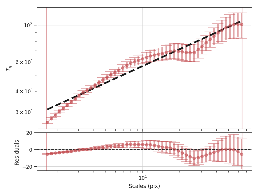
The results of the fit and a plot overlaying the fit on the transform are shown with verbose=True. The figure shows that the transform (blue diamonds) does not follow a single power-law relation across all of the scales and resulting fit (dashed blue line) is poor. The solid blue lines indicate the range of scales used in the fit. In the case of these simulated data, scales larger than about 25 pixels are affected by the edges of the map in the convolution. The flattening on scales just smaller is describing actual features in the data and may be a manifestation of the periodic box conditions; we see a similar feature with these data with the Delta-Variance as well. Unlike the Delta-Variance, the deviation from a power-law is more pronounced on scales larger than about 10 pixels. To improve the fit, we can limit the region that is fit to below this scale:
>>> wavelet = Wavelet(moment0)  # doctest: +SKIP
>>> wavelet.run(verbose=True, xlow=1 * u.pix, xhigh=10 * u.pix)  # doctest: +SKIP
                            OLS Regression Results
==============================================================================
Dep. Variable:                      y   R-squared:                       0.992
Model:                            OLS   Adj. R-squared:                  0.991
Method:                 Least Squares   F-statistic:                     2758.
Date:                Wed, 02 Aug 2017   Prob (F-statistic):           1.86e-25
Time:                        14:05:44   Log-Likelihood:                 78.364
No. Observations:                  25   AIC:                            -152.7
Df Residuals:                      23   BIC:                            -150.3
Df Model:                           1
Covariance Type:            nonrobust
==============================================================================
                 coef    std err          t      P>|t|      [0.025      0.975]
------------------------------------------------------------------------------
const          1.3279      0.006    215.931      0.000       1.315       1.341
x1             0.4946      0.009     52.516      0.000       0.475       0.514
==============================================================================
Omnibus:                        4.021   Durbin-Watson:                   0.122
Prob(Omnibus):                  0.134   Jarque-Bera (JB):                3.476
Skew:                          -0.888   Prob(JB):                        0.176
Kurtosis:                       2.572   Cond. No.                         5.95
==============================================================================
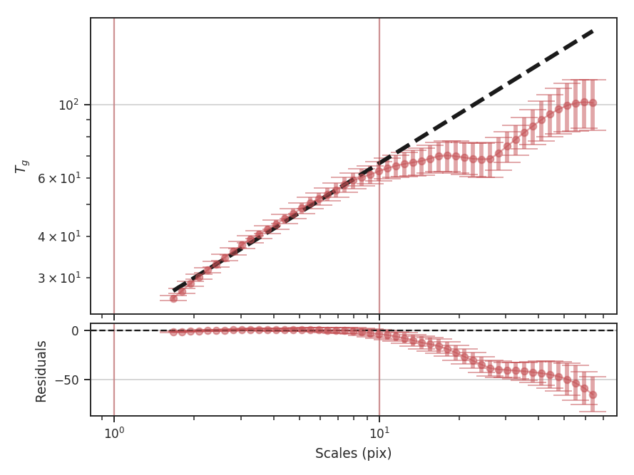
This has significantly improved the fit, and the slope of the power-law is closer to the value found from the Delta-Variance transform. The wavelet transform slope is half of the Delta-Variance slope:
>>> wavelet.slope * 2  # doctest: +SKIP
0.98916576820595215
>>> wavelet.slope_err *2  # doctest: +SKIP
0.018835675570973334
The wavelet transform gives an index of \(0.99 \pm 0.02\), while the Delta-Variance has a slope of \(1.06 \pm 0.02\) fit over a similar range. While limiting the fit gives a consistent result to other methods, the differences in the shape of the spectra may give useful information and should be interpreted carefully.
These examples have used the default scales to calculate the wavelet transforms. The default, in pixel units, will vary from 1.5 pixels to half of the smallest image dimension and will be spaced equally in logarithmic space. The number of scales to test defaults to 50; this can be changed by giving the num keyword to Wavelet. Alternatively, a custom set of scales can be given. The units of the scale can also be given in both angular and physical units (when a distance is provided). This can be useful for comparing different datasets at a common scale. For example, assume that this simulated dataset lies at a distance of 250 pc:
>>> phys_scales = np.arange(0.025, 0.5, 0.05) * u.pc
>>> wavelet = Wavelet(moment0, distance=250 * u.pc, scales=phys_scales)  # doctest: +SKIP
>>> wavelet.run(verbose=True, xlow=1 * u.pix, xhigh=10 * u.pix, xunit=u.pc)  # doctest: +SKIP
                            OLS Regression Results
==============================================================================
Dep. Variable:                      y   R-squared:                       0.983
Model:                            OLS   Adj. R-squared:                  0.977
Method:                 Least Squares   F-statistic:                     173.6
Date:                Wed, 02 Aug 2017   Prob (F-statistic):           0.000944
Time:                        14:43:07   Log-Likelihood:                 11.334
No. Observations:                   5   AIC:                            -18.67
Df Residuals:                       3   BIC:                            -19.45
Df Model:                           1
Covariance Type:            nonrobust
==============================================================================
                 coef    std err          t      P>|t|      [0.025      0.975]
------------------------------------------------------------------------------
const          1.2668      0.031     41.159      0.000       1.169       1.365
x1             0.5649      0.043     13.178      0.001       0.428       0.701
==============================================================================
Omnibus:                          nan   Durbin-Watson:                   1.633
Prob(Omnibus):                    nan   Jarque-Bera (JB):                0.461
Skew:                           0.166   Prob(JB):                        0.794
Kurtosis:                       1.549   Cond. No.                         4.25
==============================================================================
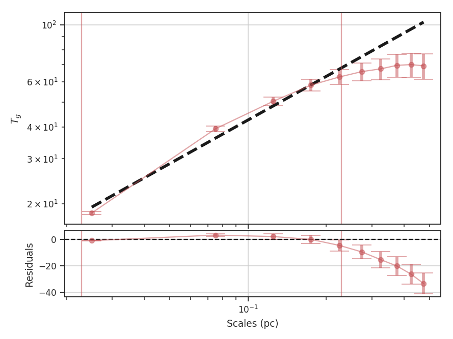
We find a similar slope using the same fit region as the previous example, though with more uncertainty since only 5 of the given scales fit into the region. Note that the plot now shows the scales in parsecs, as well. The output unit used in the plot can be changed by specifying xunit. Similarly, different units can be used in xlow and xhigh, too.
Finally, we note a difference between the TurbuStat implementation of the wavelet transform and the one described in Gill & Henriksen 1990. Their definition of the Mexican-Hat wavelet in Section 2 is an unnormalized form of the kernel and this leads to a slope of \(+2\) larger than the normalized version here. We use the Mexican-Hat implementation from the astropy.convolution package, which has the correct \(1/\pi \sigma^4\) normalization coefficient for the wavelet transform.
The \(+2\) discrepancy can be explained by thinking of the Mexican-Hat kernel as the negative of the Laplacian of a Gaussian. A normalized Gaussian has a normalization constant of \(1/2 \pi \sigma^2\), or units of \(1/{\rm length}^2\), but has a constant peak for all \(\sigma\). In order to make the Laplacian also have a constant peak, referred to as a scale-normalized derivative in image processing, we need to multiply the Mexican-Hat by a factor of \(\sigma^2\) at each scale. Combined with the normalization coefficient of \(1/\pi \sigma^4\), this restores the \(1/{\rm length}^2\) of a Gaussian (Lindeburg 1994). In order to reproduce the unnormalized version of Gill & Henriksen 1990, we need to multiply the kernel by \(\sigma^4\). To reproduce their results, we have included a normalization keyword to disable the correct normalization:
>>> wavelet = Wavelet(moment0)  # doctest: +SKIP
>>> wavelet.run(verbose=True, scale_normalization=False,
...             xhigh=10 * u.pix)  # doctest: +SKIP
                            OLS Regression Results
==============================================================================
Dep. Variable:                      y   R-squared:                       1.000
Model:                            OLS   Adj. R-squared:                  1.000
Method:                 Least Squares   F-statistic:                 7.016e+04
Date:                Wed, 02 Aug 2017   Prob (F-statistic):           1.40e-41
Time:                        15:10:40   Log-Likelihood:                 78.364
No. Observations:                  25   AIC:                            -152.7
Df Residuals:                      23   BIC:                            -150.3
Df Model:                           1
Covariance Type:            nonrobust
==============================================================================
                 coef    std err          t      P>|t|      [0.025      0.975]
------------------------------------------------------------------------------
const          1.3279      0.006    215.931      0.000       1.315       1.341
x1             2.4946      0.009    264.879      0.000       2.475       2.514
==============================================================================
Omnibus:                        4.021   Durbin-Watson:                   0.122
Prob(Omnibus):                  0.134   Jarque-Bera (JB):                3.476
Skew:                          -0.888   Prob(JB):                        0.176
Kurtosis:                       2.572   Cond. No.                         5.95
==============================================================================
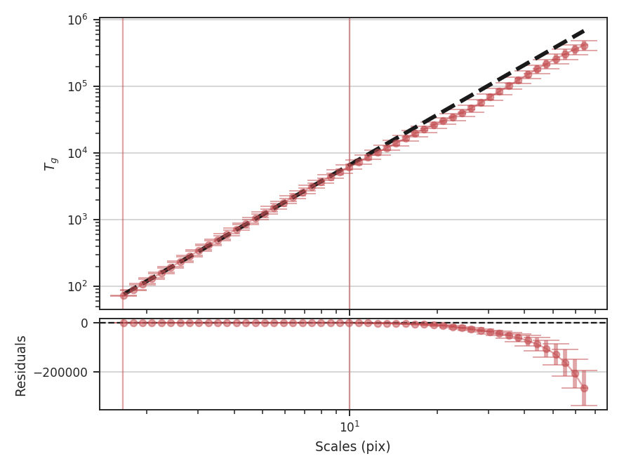
The unnormalized transform appears to follow a power-law relation over all of the scales, and when limited to the same fitting region, the fit appears to be much better. This is deceiving, however, because the extra factors of \(\sigma\) are increasing the correlation between the x and y variables in the fit! This effectively gives a slope of \(+2\) for free, regardless of the data. Further, it means that the fit statistics are no longer valid, as the underlying assumption in the model is that the y and x values are uncorrelated.
Warning
We do not recommend using the unnormalized form as it inflates the quality of the fit, hides the deviations (that may be physically relevant!), but provides no additional information or improvements.
Distance Metrics
This section describes the distance metrics defined in Koch et al. 2017 for comparing two data sets with some output of the statistics listed above. It is important to note that few of these distance metrics are defined to be absolute. Rather, most of the metrics give relative distances and are defined only when comparing with a common fiducial image.
As shown in Koch et al. 2017, the distance metrics for some statistics have more scatter than others. Some metrics also suffer from systematic issues and should be avoided when those systematics cannot be controlled for. The Cramer distance metric is an example of this; its shortcomings are described in the paper linked above, and while the implementation is still available, we recommend caution when using it.
A distance metric for Tsallis statistics has not been explored and is not currently available in this release.
Using distance metrics
Distance metrics run a statistic on two datasets and use an output of the statistic to quantitatively determine how similar the datasets are. Like the statistic classes, the distance metrics are also python classes.
Warning
Using the distance metrics requires some understanding of how the statistics are computed. Please read the introduction to using statistics page.
There is less structure in the distance metric classes compared to the statistic classes. There are two steps to using the distance metrics:
- Initialization – Like the statistics, unchanging information is given here. The two datasets are given here. However, the statistics are also run from this step, so properties often given to the
runcommand for the statistics should be given here.
Note
The distance metrics do not always use the full information from a statistic. In these cases, there will be fewer arguments to specify than the statistic’s run function.
For the Wavelet_Distance, the distance metric is initialized using:
>>> from turbustat.statistics import Wavelet_Distance
>>> from astropy.io import fits
>>> hdu = fits.open("file.fits")[0]  # doctest: +SKIP
>>> hdu2 = fits.open("file2.fits")[0]  # doctest: +SKIP
>>> wave_dist = Wavelet_Distance(hdu, hdu2, xlow=[5, 7] * u.pix,
...                              xhigh=[30, 35] * u.pix)  # doctest: +SKIP
The two datasets are given. For the wavelet transform, the distance is the absolute difference between the slopes, normalized by the square sum of the slope uncertainties. Thus it is important to set the scales that the transform is fit to. Different limits can be given for the two datasets, as shown above, by specifying xlow and xhigh with two different values. If only a single value is given, it will be used for both datasets. Most parameters that can be specified for one or both of the datasets use this format.
Alternatively, if the wavelet transform has already been computed for one or both of the datasets, the Wavelet can be passed instead of the dataset:
>>> from turbustat.statistics import Wavelet, Wavelet_Distance
>>> wave1 = Wavelet(hdu).run()  # doctest: +SKIP
>>> wave2 = Wavelet(hdu).run()  # doctest: +SKIP
>>> wave_dist = Wavelet_Distance(wave1, wave2)  # doctest: +SKIP
Some distance metrics require that the statistic be computed with a common set of bins or spatial scales. If a Wavelet is given that does not satisfy the criteria, it will be re-run with Wavelet_Distance. The criteria to avoid re-computing a statistic is specified as Notes in the distance metric docstrings. See the source code documentation on this site.
The second step is to compute the distance metric. In nearly all cases, computing the distance metric is much faster than computing the statistics. All of the distance metric classes have a
distance_metricfunction:>>> wave_dist.distance_metric(verbose=True) # doctest: +SKIP >>> wave_dist.distance # doctest: +SKIP
The distance is usually an attribute called distance. Different names are used when there are multiple distance metrics defined. For example, the PDF_Distance has hellinger_distance, ks_distance, lognormal_distance. See the source code documentation for specifics on each distance metric class. When multiple distance metrics are defined, there are often multiple functions to compute each metric. The distance_metric function will usually run all of the distance metrics.
With verbose=True in distance_metric, a summary plot showing both datasets will be returned. Usually these plots call the plotting function from the statistic classes. Labels to show in the legend for the two datasets can be given.
Note
The one metric that differs from the rest is the Cramer_Distance. This metric does not have a statistic class because it is a two-sample statistical test. The structure is the same as the rest of the distance metrics but contains more steps to compute the method.
Bispectrum Distance
See the tutorial for a description of the bispectrum.
The distance metric for the bispectrum is Bispectrum_Distance. There are two definitions of a distance:
- The surface distance is the L2 norm between the bicoherence surfaces of two 2D images:
- \[d_{\rm surface} = ||b_1(k_1, k_2) - b_2(k_1, k_2)||^2\]
The \(k_1,\,k_2\) are wavenumbers and \(b_1,\,b_2\) are the bicoherence arrays for each image.
Warning
The images must have the same shape to use this definition of distance.
- The mean distance is the absolute difference between the mean bicoherence of two 2D images:
- \[d_{\rm mean} = |\bar{b_1(k_1, k_2)} - \bar{b_1(k_1, k_2)}|\]
This distance metric can be used with images of different shapes.
The bicoherence surface is used for the distance metric because it is normalized between 0 and 1, and this normalization removes the effect of the mean of the images (meansub in the bispectrum tutorial).
More information on the distance metric definitions can be found in Koch et al. 2017
Using
The data in this tutorial are available here.
We need to import the Bispectrum_Distance class, along with a few other common packages:
>>> from turbustat.statistics import Bispectrum_Distance
>>> from astropy.io import fits
>>> import matplotlib.pyplot as plt
And we load in the two data sets; in this case, two integrated intensity (zeroth moment) maps:
>>> moment0 = fits.open("Design4_flatrho_0021_00_radmc_moment0.fits")[0]  # doctest: +SKIP
>>> moment0_fid = fits.open("Fiducial0_flatrho_0021_00_radmc_moment0.fits")[0]  # doctest: +SKIP
The images are passed to the Bispectrum_Distance class. Keyword arguments to run can also be given as the dictionary stat_kwargs. In this case, we will increase the number of random samples used to estimate the bispectrum:
>>> bispec = Bispectrum_Distance(moment0_fid, moment0,
...                              stat_kwargs={'nsamples': 10000})  # doctest: +SKIP
This call executes run for both images and may take a few minutes to run (reduce the number of samples to speed things up). Within Bispectrum_Distance is a Bispectrum for each image: bispec1 and bispec2. Each of these class instances can be run separately with, as shown in the bispectrum tutorial, to fine-tune or alter how the bispectrum is computed.
Once the bispectra are computed, we can calculate the distances between the two bispectra and create a summary plot with:
>>> bispec.distance_metric(verbose=True) # doctest: +SKIP
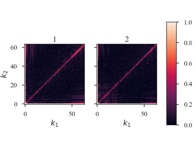
The bicoherence surfaces of both images are shown. By default, the plots are labelled with “1” and “2” in the order the data were given to Bispectrum_Distance. Custom labels can be set by setting label1 and label2 in the distance metric call.
The distances between these images are:
>>> bispec.surface_distance  # doctest: +SKIP
3.169320958026329
Since these images have equal shapes,
surface_distanceis defined. If the images do not have equal shapes, the distance will beNaN.>>> bispec.mean_distance # doctest: +SKIP 0.009241794373870557
Warning
Caution must be used when passing a pre-computed Bispectrum instead of the data for moment0 or moment0_fid as there are no checks to ensure the bispectra were computed the same way (e.g., do both have mean_sub=True set?). Ensure that the keyword arguments for the pre-computed statistic match those specified to Bispectrum_Distance. See the distance metric introduction.
Cramer Distance
The Cramer statistic was introduced by Baringhaus & Franz (2004) for multivariate two-sample testing. The statistic is defined as the difference of the Euclidean distances between the two data sets subtracted by half of the distances measured within each data set.
Yeremi et al. 2015 applied this to position-position-velocity data cubes by selecting a sample of the brightest pixels in each spectral channel to reduce the cube to a 2D data matrix. It was also used tested in Koch et al. 2017, and the definition used in TurbuStat can be found there.
Warning
Koch et al. 2017 find that this test is unsuitable for comparing data cubes that have a large difference in their mean intensities. When using this metric, be sure that the intensity distributions have similar mean intensities or apply some normalization prior to running the metric. Be cautious when interpreting these results and ensure that the distances are compared to a well-understood fiducial.
Using
The data in this tutorial are available here.
We need to import the Cramer_Distance class, along with a few other common packages:
>>> from turbustat.statistics import Cramer_Distance
>>> from astropy.io import fits
>>> import matplotlib.pyplot as plt
And we load in the two data sets. The Cramer statistic needs two cubes:
>>> cube = fits.open("Design4_flatrho_0021_00_radmc.fits")[0]  # doctest: +SKIP
>>> cube_fid = fits.open("Fiducial0_flatrho_0021_00_radmc.fits")[0]  # doctest: +SKIP
Cramer_Distance takes the two cubes as inputs. Minimum intensity values for the statistic to consider can be specified with noise_value1 and noise_value2.
>>> cramer = Cramer_Distance(cube_fid, cube, noise_value1=-np.inf,
...                          noise_value2=-np.inf)  # doctest: +SKIP
Note that, since the Cramer statistic defaults to using the upper 20% of the values in each spectral channel, there may not be large differences in the distance when the noise values are low.
The 2D data matrices and the Cramer statistic can now be calculated with:
>>> cramer.distance_metric(normalize=True, n_jobs=1, verbose=True) # doctest: +SKIP
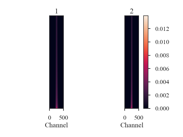
Setting verbose=True creates this figure, where the data matrices are shown for each data cube. The x-axis are the spectral channels and the y-axis are, ordered with the largest at the bottom, the largest pixel values in that spectral channel. Custom labels can be set by setting label1 and label2 in the distance metric call above.
The argument n_jobs sets how many cores to use when calculating pairwise distances with the sklearn paired_distances function. This is the slowest step in computing the Cramer statistic; see format_data for more information.
The distance between the data cubes is:
>>> cramer.distance  # doctest: +SKIP
0.18175851051788378
distance_metric performs two steps: format_data to find the 2D data matrix for each cube, and cramer_statistic to calculate the distance. These steps can be run separately to allow for changes in the keyword arguments of both.
Delta-Variance Distance
See the tutorial for a description of Delta-Variance.
The distance metric for Delta-Variance is DeltaVariance_Distance. There are two definitions of a distance:
- The curve distance is the L2 norm between the delta-variance curves normalized by the sum of each curve:
- \[d_{curve} = \left|\left|\frac{\sigma_{\Delta,1}^2 (\ell)}{\sum_i \sigma_{\Delta,1}^2 (\ell)} - \frac{\sigma_{\Delta,2}^2 (\ell)}{\sum_i \sigma_{\Delta,2}^2 (\ell)}\right|\right|\]
\(\sigma_{\Delta,i}\) are the delta-variance values at lag \(\ell\).
This is a non-parametric attempt to describe the entire delta-variance curve, including regions that are not well fit by a power-law model.
Warning
This distance requires the delta-variance to be measured at the same lags in angular units. This is described further below.
- The slope distance is the t-statistic of the difference in the fitted slopes:
- \[d_{\rm slope} = \frac{|\beta_1 - \beta_2|}{\sqrt{\sigma_{\beta_1}^2 + \sigma_{\beta_1}^2}}\]
\(\beta_i\) are the slopes of the delta-variance curves and \(\sigma_{\beta_i}\) are the uncertainty of the slopes.
More information on the distance metric definitions can be found in Koch et al. 2017
Using
The data in this tutorial are available here.
We need to import the DeltaVariance_Distance class, along with a few other common packages:
>>> from turbustat.statistics import DeltaVariance_Distance
>>> from astropy.io import fits
>>> import matplotlib.pyplot as plt
And we load in the two data sets; in this case, two integrated intensity (zeroth moment) maps:
>>> moment0 = fits.open("Design4_flatrho_0021_00_radmc_moment0.fits")[0]  # doctest: +SKIP
>>> moment0_fid = fits.open("Fiducial0_flatrho_0021_00_radmc_moment0.fits")[0]  # doctest: +SKIP
The error maps are saved in the second extension of these FITS files. These can be used as weights for the Delta-Variance:
>>> moment0_err = fits.open("Design4_flatrho_0021_00_radmc_moment0.fits")[1]  # doctest: +SKIP
>>> moment0_fid_err = fits.open("Fiducial0_flatrho_0021_00_radmc_moment0.fits")[1]  # doctest: +SKIP
The images (and optionally the error maps) are passed to the DeltaVariance_Distance class:
>>> delvar = DeltaVariance_Distance(moment0_fid, moment0, weights1=moment0_err,
...                                weights2=moment0_fid_err)  # doctest: +SKIP
>>> delvar.distance_metric(verbose=True, xunit=u.pix)  # doctest: +SKIP
                            WLS Regression Results
==============================================================================
Dep. Variable:                      y   R-squared:                       0.688
Model:                            WLS   Adj. R-squared:                  0.674
Method:                 Least Squares   F-statistic:                     11.70
Date:                Thu, 01 Nov 2018   Prob (F-statistic):            0.00234
Time:                        13:32:37   Log-Likelihood:                 4.9953
No. Observations:                  25   AIC:                            -5.991
Df Residuals:                      23   BIC:                            -3.553
Df Model:                           1
Covariance Type:                  HC3
==============================================================================
                 coef    std err          z      P>|z|      [0.025      0.975]
------------------------------------------------------------------------------
const          2.5660      0.155     16.602      0.000       2.263       2.869
x1             0.6353      0.186      3.421      0.001       0.271       0.999
==============================================================================
Omnibus:                        3.845   Durbin-Watson:                   0.313
Prob(Omnibus):                  0.146   Jarque-Bera (JB):                3.114
Skew:                          -0.858   Prob(JB):                        0.211
Kurtosis:                       2.784   Cond. No.                         7.05
==============================================================================
                            WLS Regression Results
==============================================================================
Dep. Variable:                      y   R-squared:                       0.956
Model:                            WLS   Adj. R-squared:                  0.954
Method:                 Least Squares   F-statistic:                     66.34
Date:                Thu, 01 Nov 2018   Prob (F-statistic):           3.15e-08
Time:                        13:32:37   Log-Likelihood:                 14.779
No. Observations:                  25   AIC:                            -25.56
Df Residuals:                      23   BIC:                            -23.12
Df Model:                           1
Covariance Type:                  HC3
==============================================================================
                 coef    std err          z      P>|z|      [0.025      0.975]
------------------------------------------------------------------------------
const          1.6490      0.118     14.001      0.000       1.418       1.880
x1             1.3072      0.160      8.145      0.000       0.993       1.622
==============================================================================
Omnibus:                        0.251   Durbin-Watson:                   0.559
Prob(Omnibus):                  0.882   Jarque-Bera (JB):                0.394
Skew:                           0.195   Prob(JB):                        0.821
Kurtosis:                       2.523   Cond. No.                         10.8
==============================================================================
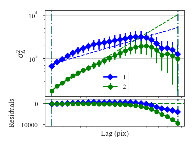
A summary of the fits are printed along with a plot of the two delta-variance curves and the fit residuals when verbose=True. Custom labels can be set by setting label1 and label2 in the distance metric call.
The distances between these two datasets are:
>>> delvar.curve_distance  # doctest: +SKIP
0.8374744762224977
>>> delvar.slope_distance  # doctest: +SKIP
2.737516700717662
In this case, the default settings were used and all portions of the delta-variance curves were used in the fit, yielding poor fits. Setting can be passed to run by specifying inputs to delvar_kwargs. For example, we will now limit the Delta-Variance fitting between 4 and 10 pixel lags:
>>>  delvar_fit = DeltaVariance_Distance(moment0_fid, moment0, weights1=moment0_err,
...                                      weights2=moment0_fid_err,
...                                      delvar_kwargs={'xlow': 4 * u.pix,
...                                                     'xhigh': 10 * u.pix})  # doctest: +SKIP
>>> delvar_fit.distance_metric(verbose=True, xunit=u.pix)  # doctest: +SKIP
                            WLS Regression Results
==============================================================================
Dep. Variable:                      y   R-squared:                       0.985
Model:                            WLS   Adj. R-squared:                  0.982
Method:                 Least Squares   F-statistic:                     77.59
Date:                Thu, 01 Nov 2018   Prob (F-statistic):           0.000313
Time:                        13:32:37   Log-Likelihood:                 20.519
No. Observations:                   7   AIC:                            -37.04
Df Residuals:                       5   BIC:                            -37.15
Df Model:                           1
Covariance Type:                  HC3
==============================================================================
                 coef    std err          z      P>|z|      [0.025      0.975]
------------------------------------------------------------------------------
const          2.4484      0.087     28.186      0.000       2.278       2.619
x1             0.9605      0.109      8.809      0.000       0.747       1.174
==============================================================================
Omnibus:                          nan   Durbin-Watson:                   0.931
Prob(Omnibus):                    nan   Jarque-Bera (JB):                0.657
Skew:                          -0.378   Prob(JB):                        0.720
Kurtosis:                       1.704   Cond. No.                         16.7
==============================================================================
                            WLS Regression Results
==============================================================================
Dep. Variable:                      y   R-squared:                       0.995
Model:                            WLS   Adj. R-squared:                  0.994
Method:                 Least Squares   F-statistic:                     206.3
Date:                Thu, 01 Nov 2018   Prob (F-statistic):           2.95e-05
Time:                        13:32:37   Log-Likelihood:                 23.185
No. Observations:                   7   AIC:                            -42.37
Df Residuals:                       5   BIC:                            -42.48
Df Model:                           1
Covariance Type:                  HC3
==============================================================================
                 coef    std err          z      P>|z|      [0.025      0.975]
------------------------------------------------------------------------------
const          1.7989      0.065     27.823      0.000       1.672       1.926
x1             1.1402      0.079     14.363      0.000       0.985       1.296
==============================================================================
Omnibus:                          nan   Durbin-Watson:                   1.289
Prob(Omnibus):                    nan   Jarque-Bera (JB):                0.654
Skew:                           0.062   Prob(JB):                        0.721
Kurtosis:                       1.507   Cond. No.                         16.6
==============================================================================
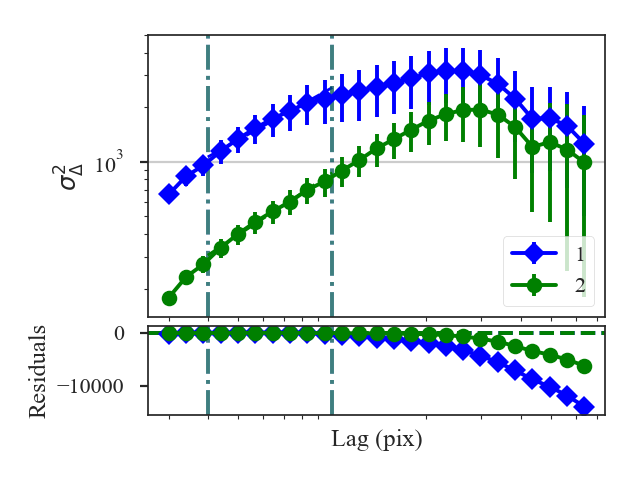
The fits are improved, particularly for the first data set (moment0_fid), with the limits specified. Both of the distances are changed: the slope distance from the improved fits and curve distance because the comparison is limited to the fit limits:
>>> delvar_fit.curve_distance  # doctest: +SKIP
0.06769078224562503
>>> delvar_fit.slope_distance  # doctest: +SKIP
1.3324272202721044
What if you want to set different limits for the two datasets? Or how can you handle datasets with different boundary conditions in the convolution (i.e., observations vs simulated observations)? A second set of kwargs can be given with delvar2_kwargs, which specifies the parameters for the second dataset. For example, to pass a different set of fit limits for the second dataset (moment0):
>>>  delvar_fitdiff = DeltaVariance_Distance(moment0_fid, moment0, weights1=moment0_err,
...                                          weights2=moment0_fid_err,
...                                          delvar_kwargs={'xlow': 4 * u.pix,
...                                                         'xhigh': 10 * u.pix},
...                                          delvar2_kwargs={'xlow': 6 * u.pix,
...                                                          'xhigh': 20 * u.pix})  # doctest: +SKIP
>>> delvar_fitdiff.distance_metric(verbose=True, xunit=u.pix)  # doctest: +SKIP
                            WLS Regression Results
==============================================================================
Dep. Variable:                      y   R-squared:                       0.985
Model:                            WLS   Adj. R-squared:                  0.982
Method:                 Least Squares   F-statistic:                     77.59
Date:                Thu, 01 Nov 2018   Prob (F-statistic):           0.000313
Time:                        13:32:38   Log-Likelihood:                 20.519
No. Observations:                   7   AIC:                            -37.04
Df Residuals:                       5   BIC:                            -37.15
Df Model:                           1
Covariance Type:                  HC3
==============================================================================
                 coef    std err          z      P>|z|      [0.025      0.975]
------------------------------------------------------------------------------
const          2.4484      0.087     28.186      0.000       2.278       2.619
x1             0.9605      0.109      8.809      0.000       0.747       1.174
==============================================================================
Omnibus:                          nan   Durbin-Watson:                   0.931
Prob(Omnibus):                    nan   Jarque-Bera (JB):                0.657
Skew:                          -0.378   Prob(JB):                        0.720
Kurtosis:                       1.704   Cond. No.                         16.7
==============================================================================
                            WLS Regression Results
==============================================================================
Dep. Variable:                      y   R-squared:                       0.999
Model:                            WLS   Adj. R-squared:                  0.999
Method:                 Least Squares   F-statistic:                 1.084e+04
Date:                Thu, 01 Nov 2018   Prob (F-statistic):           1.99e-12
Time:                        13:32:38   Log-Likelihood:                 36.872
No. Observations:                   9   AIC:                            -69.74
Df Residuals:                       7   BIC:                            -69.35
Df Model:                           1
Covariance Type:                  HC3
==============================================================================
                 coef    std err          z      P>|z|      [0.025      0.975]
------------------------------------------------------------------------------
const          1.8957      0.010    198.429      0.000       1.877       1.914
x1             1.0257      0.010    104.110      0.000       1.006       1.045
==============================================================================
Omnibus:                        0.438   Durbin-Watson:                   3.074
Prob(Omnibus):                  0.803   Jarque-Bera (JB):                0.436
Skew:                           0.381   Prob(JB):                        0.804
Kurtosis:                       2.237   Cond. No.                         16.6
==============================================================================
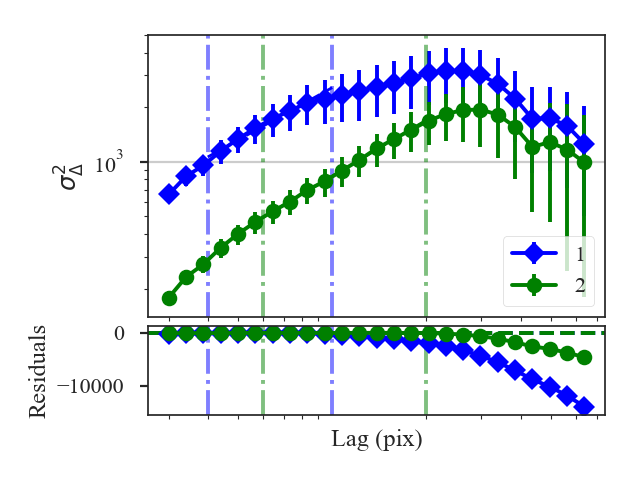
The fit limits, shown with the dot-dashed vertical lines in the plot, differ between the datasets. This will change the slope distance:
>>> delvar_fit.slope_distance  # doctest: +SKIP
0.5956856398497301
But the curve distance is no longer defined:
>>> delvar_fit.curve_distance  # doctest: +SKIP
nan
The curve distance is only valid when the same set of lags are used to compute the delta-variance. Thus having different fit limits violates this condition and the distance is returned as a nan.
The curve distance will also be undefined if different sets of lags are used for the datasets. By default, use_common_lags=True is used in DeltaVariance_Distance, which will find a common set of scales in angular units between the two datasets.
For further fine-tuning of the delta-variance for either dataset, the DeltaVariance classes for each dataset can be accessed as delvar1 and delvar2. Each of these class instances can be run separately, as shown in the delta-variance tutorial, to fine-tune or alter how the delta-variance is computed.
Dendrogram Distance
See the tutorial for a description of the dendrogram statistics.
Warning
Requires the optional astrodendro package to be installed. See the documentation
Using the two comparisons defined by Burkhart et al. 2013, Dendro_Distance provides two distance metrics:
The distance between histograms of peak intensity in the leaves of the dendrogram, measured over a range of minimum branch heights, is:
\[d_{\mathrm{Hist}} = \left[\sum H(p_{1,\delta_I},p_{2,\delta_I})\right]/N_\delta\]\(p_{i,\delta_I}\) are the histograms with minimum branch height of \(\delta_I\), \(H(i, j)\) is the Hellinger distance, and \(N_{\delta}\) is the number of branch heights (and histograms) that the dendrogram was computed for.
The slopes of the linear relation fit to the log of the number of features in the tree as a function of minimum branch height:
\[d_{\rm slope} = \frac{|\beta_1 - \beta_2|}{\sqrt{\sigma_{\beta_1}^2 + \sigma_{\beta_1}^2}}\]\(\beta_i\) are the slopes of the fitted lines and \(\sigma_{\beta_i}\) are the uncertainty of the slopes.
More information on the distance metric definitions can be found in Koch et al. 2017
Using
The data in this tutorial are available here.
We need to import the Dendrogram_Distance class, along with a few other common packages:
>>> from turbustat.statistics import Dendrogram_Distance
>>> from astropy.io import fits
>>> import matplotlib.pyplot as plt
And we load in the two data sets. Dendrogram_Distance can be given two 2D images or cubes. For this example, we will use two cubes:
>>> cube = fits.open("Design4_flatrho_0021_00_radmc.fits")[0]  # doctest: +SKIP
>>> cube_fid = fits.open("Fiducial0_flatrho_0021_00_radmc.fits")[0]  # doctest: +SKIP
Dendrogram_Distance requires the two datasets to be given. A number of other parameters can be specified to control the dendrogram settings or fitting settings. This example sets the minimum deltas (branch height) for the dendrograms, as explained in the dendrogram tutorial. Other dendrogram settings, such as the minimum pixel intensity to use and the minimum number of pixels per structure, are also set.
>>> dend_dist = Dendrogram_Distance(cube_fid, cube,
...                                 min_deltas=np.logspace(-2, 0, 50),
...                                 min_features=100,
...                                 dendro_params={"min_value": 0.005,
...                                                "min_npix": 50})  # doctest: +SKIP
The min_features sets a threshold on the number of ‘features’ in a dendrogram needed for it to be included to calculate the distances. “Features” is the number of branches and leaves in the dendrogram. As delta is increased in the dendrogram, the number of features drops significantly, with large values leaving only a few features in the dendrogram. min_features ensures a meaningful histogram can be measured from the dendrogram properties.
If additional parameters need to be set to create the dendrograms, dendro_kwargs takes a dictionary as input and passes the arguments to run. Separate settings can be given for each dataset by specifying both dendro_kwargs and dendro2_kwargs. The individual Dendrogram_Stats objects can be also be accessed as dendro1 and dendro2 (see the dendrogram tutorial for more information).
- To calculate the two dendrogram distances, we run:
>>> dend_dist.distance_metric(verbose=True) # doctest: +SKIP
The distance computation is very fast for both methods so both distance metrics are always computed.
Verbose mode creates two plots, which can be saved by specifying save_name in the call above. The first plot shows the histograms used in the Hellinger distance.
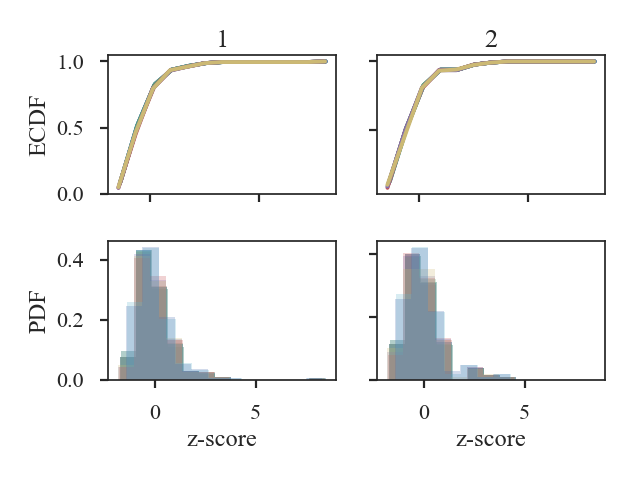
The top two panels are the ECDFs of the histograms of peak intensity within features (branches or leaves) of the dendrogram. The histograms are shown in the bottom two panels. The first dataset is shown in the first column plots and the second in the second column plots. Note that the intensity values are standardized in all plots. There are several curves/histograms shown in each plot. Each one is the dendrogram with different cut-offs of the minimum delta (branch height).
The histogram distance is:
>>> dend_dist.histogram_distance  # doctest: +SKIP
0.14298381514818145
The second plot shows the log of the number of features (branches + leaves) in a dendrogram as a function of log delta (minimum branch height):
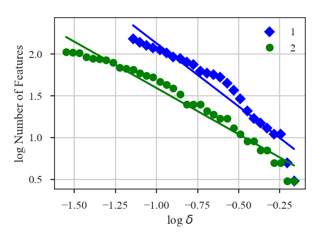
A line is fit to this relation, and the difference in the slopes of those lines is used to calculate the distance:
>>> dend_dist.num_distance  # doctest: +SKIP
2.7987025053709766
For both plots, the plotting labels can be changed from 1 and 2 by setting label1 and label2 in distance_metric.
For large data sets, creating the dendrogram can be slow. Particularly when comparing many datasets to a fiducial dataset, recomputing the dendrogram each time wastes a lot of time. Dendrogram_Distance can be passed a precomputed Dendrogram_Stats instead of giving a dataset. See the distance metric introduction.
Warning
The saved dendrograms should be run with the same min_deltas given to Dendrogram_Stats. The histogram distance is only valid when comparing dendrograms measured with the same deltas.
Genus Distance
See the tutorial for a description of Genus statistics.
The distance metric for Genus is Genus_Distance. The distance between the Genus curves is defined as:
where \(G_{j}\left(I_{0, i}\right)\) are the Genus curves, and \(A_{j}\) is the total area each Genus curve is measured over to normalize comparisons of images of different sizes.
More information on the distance metric definitions can be found in Koch et al. 2017
Using
The data in this tutorial are available here.
We need to import the Genus_Distance class, along with a few other common packages:
>>> from turbustat.statistics import Genus_Distance
>>> from astropy.io import fits
>>> import astropy.units as u
>>> import numpy as np
And we load in the two data sets; in this case, two integrated intensity (zeroth moment) maps:
>>> moment0 = fits.open("Design4_flatrho_0021_00_radmc_moment0.fits")[0]  # doctest: +SKIP
>>> moment0_fid = fits.open("Fiducial0_flatrho_0021_00_radmc_moment0.fits")[0]  # doctest: +SKIP
The two images are passed to the Genus_Distance class:
>>> genus = Genus_Distance(moment0_fid, moment0,
...                        lowdens_percent=15, highdens_percent=85, numpts=100,
...                        genus_kwargs=dict(min_size=4 * u.pix**2))  # doctest: +SKIP
Genus_Distance accepts similar keyword arguments to Genus. Keywords to run can be specified in a dictionary to genus_kwargs. Separate keywords for the second image (moment0) can be specified in a second dictionary to genus2_kwargs.
To find the distance between the images:
>>> genus.distance_metric(verbose=True) # doctest: +SKIP
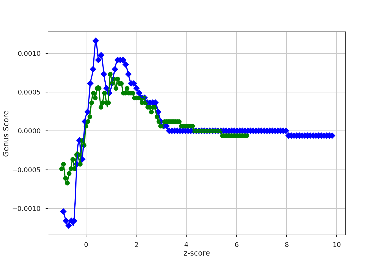
This returns a figure that plots the Genus curves of the two images, where the image values are standardized (zero mean and standard deviation of one). Colours, labels, and symbols in the plot can be changed. See distance_metric.
When comparing many images to a fiducial image, a pre-computed Genus can be passed instead of a dataset. See the distance metric introduction.
MVC Distance
See the tutorial for a description of Modified Velocity Centroids (MVC).
The distance metric for MVC is based on the t-statistics of the difference between the power spectrum slopes:
\(\beta_i\) and \(\sigma_{\beta_i}\) is the index and index uncertainty, respectively.
More information on the distance metric definitions can be found in Koch et al. 2017.
Using
The data in this tutorial are available here.
We need to import the MVC_Distance class, along with a few other common packages:
>>> from turbustat.statistics import MVC_Distance
>>> from astropy.io import fits
>>> import matplotlib.pyplot as plt
MVC is the only (current) statistic in TurbuStat that requires multiple moment arrays. Because of this, the input for MVC_Distance has a different format than the other distance metrics: a dictionary that contains the array and headers:
>>> moment0 = fits.open("Design4_flatrho_0021_00_radmc_moment0.fits")[0]  # doctest: +SKIP
>>> centroid = fits.open("Design4_flatrho_0021_00_radmc_centroid.fits")[0]  # doctest: +SKIP
>>> lwidth = fits.open("Design4_flatrho_0021_00_radmc_linewidth.fits")[0]  # doctest: +SKIP
>>> data = {"moment0": [moment0.data, moment0.header],
...         "centroid": [centroid.data, centroid.header],
...         "linewidth": [lwidth.data, lwidth.header]}  # doctest: +SKIP
And we create a second dictionary for the data set to compare with:
>>> moment0_fid = fits.open("Fiducial0_flatrho_0021_00_radmc_moment0.fits")[0]  # doctest: +SKIP
>>> centroid_fid = fits.open("Fiducial0_flatrho_0021_00_radmc_centroid.fits")[0]  # doctest: +SKIP
>>> lwidth_fid = fits.open("Fiducial0_flatrho_0021_00_radmc_linewidth.fits")[0]  # doctest: +SKIP
>>> data_fid = {"moment0": [moment0.data, moment0.header],
...             "centroid": [centroid.data, centroid.header],
...             "linewidth": [lwidth.data, lwidth.header]}  # doctest: +SKIP
These dictionaries can optionally include uncertainty arrays for the moments using the same format with keywords moment0_error, centroid_error, and linewidth_error.
These dictionaries get passed to MVC_Distance:
>>> mvc = MVC_Distance(data_fid, data) # doctest: +SKIP
To calculate the distance between the MVC power-spectra is calculated with:
>>> mvc.distance_metric(verbose=True, xunit=u.pix**-1)  # doctest: +SKIP
                            OLS Regression Results
==============================================================================
Dep. Variable:                      y   R-squared:                       0.925
Model:                            OLS   Adj. R-squared:                  0.924
Method:                 Least Squares   F-statistic:                     378.5
Date:                Tue, 13 Nov 2018   Prob (F-statistic):           8.18e-34
Time:                        10:21:40   Log-Likelihood:                -62.343
No. Observations:                  91   AIC:                             128.7
Df Residuals:                      89   BIC:                             133.7
Df Model:                           1
Covariance Type:                  HC3
==============================================================================
                 coef    std err          z      P>|z|      [0.025      0.975]
------------------------------------------------------------------------------
const         15.2461      0.161     94.965      0.000      14.931      15.561
x1            -4.8788      0.251    -19.455      0.000      -5.370      -4.387
==============================================================================
Omnibus:                        5.193   Durbin-Watson:                   0.068
Prob(Omnibus):                  0.075   Jarque-Bera (JB):                4.522
Skew:                          -0.459   Prob(JB):                        0.104
Kurtosis:                       2.408   Cond. No.                         4.40
==============================================================================
                            OLS Regression Results
==============================================================================
Dep. Variable:                      y   R-squared:                       0.941
Model:                            OLS   Adj. R-squared:                  0.941
Method:                 Least Squares   F-statistic:                     477.5
Date:                Tue, 13 Nov 2018   Prob (F-statistic):           1.55e-37
Time:                        10:21:40   Log-Likelihood:                -52.867
No. Observations:                  91   AIC:                             109.7
Df Residuals:                      89   BIC:                             114.8
Df Model:                           1
Covariance Type:                  HC3
==============================================================================
                 coef    std err          z      P>|z|      [0.025      0.975]
------------------------------------------------------------------------------
const         14.0302      0.144     97.714      0.000      13.749      14.312
x1            -5.0144      0.229    -21.853      0.000      -5.464      -4.565
==============================================================================
Omnibus:                        3.541   Durbin-Watson:                   0.129
Prob(Omnibus):                  0.170   Jarque-Bera (JB):                3.488
Skew:                          -0.469   Prob(JB):                        0.175
Kurtosis:                       2.800   Cond. No.                         4.40
==============================================================================
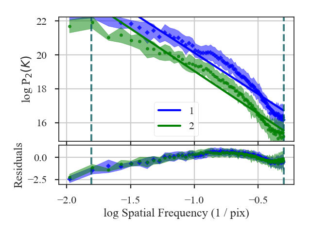
The MVC spectra are plotted in the figure and the fit summaries are printed out. The distance between the indices is:
>>> mvc.distance  # doctest: +SKIP
0.3988169606167437
This is an awful fit. We want to limit where the spectra are fit. Keywords for MVC can be passed with low_cut, high_cut, breaks, pspec_kwargs and pspec2_kwargs. If separate parameters need to be set, a two-element list or array can be given to low_cut, high_cut and breaks; the second element will be used for the second data set. For example, limiting the fit region can be done with:
>>> mvc = MVC_Distance(data_fid, data, low_cut=0.02 / u.pix,
...                    high_cut=0.4 / u.pix)  # doctest: +SKIP
>>> mvc.distance_metric(verbose=True, xunit=u.pix**-1)  # doctest: +SKIP
                            OLS Regression Results
==============================================================================
Dep. Variable:                      y   R-squared:                       0.946
Model:                            OLS   Adj. R-squared:                  0.942
Method:                 Least Squares   F-statistic:                     135.6
Date:                Tue, 13 Nov 2018   Prob (F-statistic):           2.99e-08
Time:                        10:36:41   Log-Likelihood:                 10.700
No. Observations:                  15   AIC:                            -17.40
Df Residuals:                      13   BIC:                            -15.98
Df Model:                           1
Covariance Type:                  HC3
==============================================================================
                 coef    std err          z      P>|z|      [0.025      0.975]
------------------------------------------------------------------------------
const         17.9988      0.266     67.588      0.000      17.477      18.521
x1            -2.5502      0.219    -11.647      0.000      -2.979      -2.121
==============================================================================
Omnibus:                        1.189   Durbin-Watson:                   2.376
Prob(Omnibus):                  0.552   Jarque-Bera (JB):                0.814
Skew:                          -0.200   Prob(JB):                        0.666
Kurtosis:                       1.931   Cond. No.                         13.5
==============================================================================
                            OLS Regression Results
==============================================================================
Dep. Variable:                      y   R-squared:                       0.951
Model:                            OLS   Adj. R-squared:                  0.948
Method:                 Least Squares   F-statistic:                     70.08
Date:                Tue, 13 Nov 2018   Prob (F-statistic):           1.36e-06
Time:                        10:36:41   Log-Likelihood:                 10.420
No. Observations:                  15   AIC:                            -16.84
Df Residuals:                      13   BIC:                            -15.42
Df Model:                           1
Covariance Type:                  HC3
==============================================================================
                 coef    std err          z      P>|z|      [0.025      0.975]
------------------------------------------------------------------------------
const         16.7135      0.390     42.879      0.000      15.950      17.477
x1            -2.7335      0.327     -8.371      0.000      -3.373      -2.094
==============================================================================
Omnibus:                        0.831   Durbin-Watson:                   2.076
Prob(Omnibus):                  0.660   Jarque-Bera (JB):                0.621
Skew:                          -0.449   Prob(JB):                        0.733
Kurtosis:                       2.568   Cond. No.                         13.5
==============================================================================
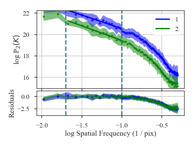
The distance is now:
>>> mvc.distance  # doctest: +SKIP
0.46621655722371613
A pre-computed MVC class can also be passed instead of giving a dataset as the input. See the distance metric introduction.
PCA Distance
See the tutorial for a description of Principal Component Analysis (PCA).
We define the PCA distance as the L2 distance between the normalized eigenvalues of two spectral-line data cubes:
The normalized eigenvalues are \(\lambda_{i} / \sum_i \lambda_{i}\).
More information on the distance metric definitions can be found in Koch et al. 2017.
Using
The data in this tutorial are available here.
We need to import the PCA_Distance class, along with a few other common packages:
>>> from turbustat.statistics import PCA_Distance
>>> from astropy.io import fits
>>> import matplotlib.pyplot as plt
PCA_Distance takes two data cubes as input:
>>> cube = fits.open("Design4_flatrho_0021_00_radmc.fits")[0]  # doctest: +SKIP
>>> cube_fid = fits.open("Fiducial0_flatrho_0021_00_radmc.fits")[0]  # doctest: +SKIP
>>> pca = PCA_Distance(cube_fid, cube, n_eigs=50, mean_sub=True)  # doctest: +SKIP
There are two additional keywords that set the number of eigenvalues to include in the distance calculation (n_eigs), and whether to subtract the mean from each spectral channel (mean_sub).
To calculate the distance between the eigenvalues:
>>> pca.distance_metric(verbose=True)  # doctest: +SKIP
Proportions of total variance: 1 - 1.000, 2 - 1.000
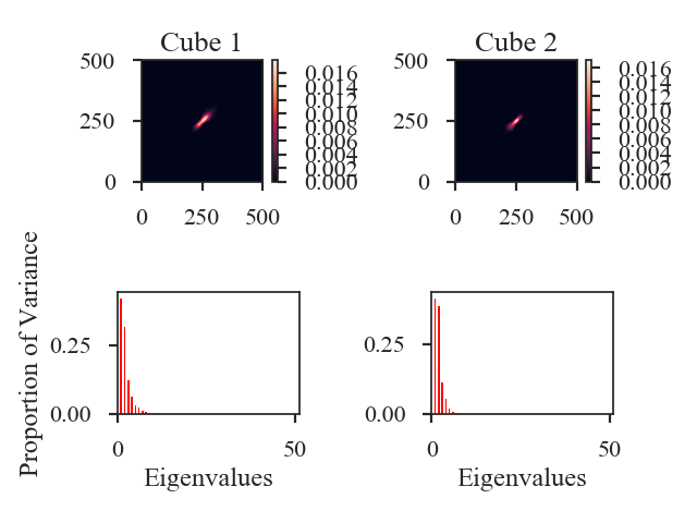
This prints out what fraction of the total variance is included in the eigenvalue vectors for each data cube. The image shows the covariance matrix for each data cube in the first row and a bar chart of the eigenvalues in the second row.
And the distance is:
>>> pca.distance  # doctest: +SKIP
0.07211706060387167
Note that a comparison of the size-line width from PCA as a distance metric is not yet implemented.
A pre-computed PCA class can also be passed instead of a dataset. See the distance metric introduction.
PDF Distance
See the tutorial for a description of PDFs.
There are multiple ways to define the distance between PDFs. Two of the metrics are non-parametric:
- The Hellinger distance between the PDFs (computed over the same set of bins):
- \[d_{\rm Hellinger}(p_1,p_2) = \frac{1}{\sqrt{2}}\left\{\sum_{\tilde{I}} \left[ \sqrt{p_1(\tilde{I})} - \sqrt{p_{2}(\tilde{I})} \right]^2\right\}^{1/2}.\]
where \(p_i\) are the histogram values at the bin \(\tilde{I}\).
- The Kolmogorov-Smirnov Distance between the ECDFs of the PDFs:
- \[d_{\rm KS}(P_1, P_2) = {\rm sup} \left| P_1(\tilde{I}) - P_2(\tilde{I}) \right|\]
where \(P_i\) is the ECDF at the value \(\tilde{I}\).
There is also one parametric distance metric included in PDF_Distance: the t-statistic of the difference in the fitted log-normal widths:
where \(w_i\) is the width of the log-normal distribution fit.
More information on the distance metric definitions can be found in Koch et al. 2017.
Using
The data in this tutorial are available here.
We need to import the PDF_Distance class, along with a few other common packages:
>>> from turbustat.statistics import PDF_Distance
>>> from astropy.io import fits
>>> import matplotlib.pyplot as plt
And we load in the two data sets. PDF_Distance can be given two 2D images or cubes. For this example, we will use two integrated intensity images:
>>> moment0 = fits.open(osjoin(data_path, "Design4_flatrho_0021_00_radmc_moment0.fits"))[0]
>>> moment0_fid = fits.open(osjoin(data_path, "Fiducial0_flatrho_0021_00_radmc_moment0.fits"))[0]
These two images are given as the inputs to PDF_Distance. Other parameters can be set here, including the minimum images values to be included in the histograms (min_val1/min_val2), whether to fit a log-normal distribution (do_fit), and what type of normalization to use on the data (normalization_type; see the PDF tutorial):
>>> pdf = PDF_Distance(moment0_fid, moment0, min_val1=0.0, min_val2=0.0,
...                    do_fit=True, normalization_type=None)  # doctest: +SKIP
This will create and run two PDF instances using a common set of bins for the histograms. These can be accessed as pdf1 and pdf2.
To calculate the distances, we run:
>>> pdf.distance_metric(verbose=True)  # doctest: +SKIP
Optimization terminated successfully.
         Current function value: 6.335450
         Iterations: 36
         Function evaluations: 72
Optimization terminated successfully.
         Current function value: 6.007851
         Iterations: 34
         Function evaluations: 69
                              Likelihood Results
==============================================================================
Dep. Variable:                      y   Log-Likelihood:            -1.0380e+05
Model:                     Likelihood   AIC:                         2.076e+05
Method:            Maximum Likelihood   BIC:                         2.076e+05
Date:                Wed, 14 Nov 2018
Time:                        09:58:10
No. Observations:               16384
Df Residuals:                   16382
Df Model:                           2
==============================================================================
                 coef    std err          z      P>|z|      [0.025      0.975]
------------------------------------------------------------------------------
par0           0.4553      0.003    181.019      0.000       0.450       0.460
par1         299.8377      1.067    281.114      0.000     297.747     301.928
==============================================================================
                              Likelihood Results
==============================================================================
Dep. Variable:                      y   Log-Likelihood:                -98433.
Model:                     Likelihood   AIC:                         1.969e+05
Method:            Maximum Likelihood   BIC:                         1.969e+05
Date:                Wed, 14 Nov 2018
Time:                        09:58:10
No. Observations:               16384
Df Residuals:                   16382
Df Model:                           2
==============================================================================
                 coef    std err          z      P>|z|      [0.025      0.975]
------------------------------------------------------------------------------
par0           0.4360      0.002    181.019      0.000       0.431       0.441
par1         225.6771      0.769    293.602      0.000     224.171     227.184
==============================================================================
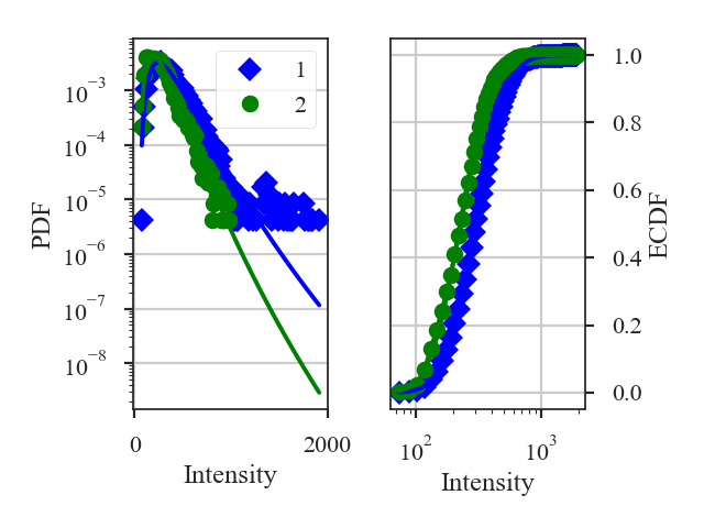
This returns a summary of the log-normal fits (if do_fit=True) and a plot of the PDF and ECDF of each data set. The solid lines in the plot are the fitted distributions.
By default, all three distance metrics are run. For these images, the distances are:
>>> pdf.hellinger_distance  # doctest: +SKIP
0.23007068347013115
>>> pdf.ks_distance  # doctest: +SKIP
0.24285888671875
>>> pdf.lognormal_distance  # doctest: +SKIP
5.561198154785891
Each distance metric can be run separately by running its function in PDF_Distance, or by setting the statistic keyword in distance_metric.
Because of the Hellinger distance requires that the PDF histograms have the same bins, there is no input to give a pre-computed fiducial PDF, unlike most of the other distance metric classes.
Spatial Power Spectrum Distance
See the tutorial for a description of the spatial power-spectrum.
The distance metric for the power-spectrum is PSpec_Distance. The distance is defined as the t-statistic between the indices of the power-spectra:
\(\beta_i\) are the slopes of the power-spectra and \(\sigma_{\beta_i}\) are the uncertainties.
More information on the distance metric definitions can be found in Koch et al. 2017
Using
The data in this tutorial are available here.
We need to import the Pspec_Distance class, along with a few other common packages:
>>> from turbustat.statistics import PSpec_Distance
>>> from astropy.io import fits
>>> import matplotlib.pyplot as plt
>>> import astropy.units as u
And we load in the two data sets; in this case, two integrated intensity (zeroth moment) maps:
>>> moment0 = fits.open("Design4_flatrho_0021_00_radmc_moment0.fits")[0]  # doctest: +SKIP
>>> moment0_fid = fits.open("Fiducial0_flatrho_0021_00_radmc_moment0.fits")[0]  # doctest: +SKIP
These two images are given as inputs to Pspec_Distance. We know from the power-spectrum tutorial that there should be limits set on where the power-spectra are fit. These can be specified with low_cut and high_cut, along with breaks if the power-spectrum is best fit with a broken power-law model. In this case, we will use the same fit limits for both power-spectra, but separate limits can be given for each image by giving a two-element list to any of these three keywords.
>>> pspec = PSpec_Distance(moment0_fid, moment0,
... low_cut=0.025 / u.pix, high_cut=0.1 / u.pix,) # doctest: +SKIP
This will create and run two PowerSpectrum instances, which can be accessed as pspec1 and pspec2.
To find the distance between these two images, we run:
>>> pspec.distance_metric(verbose=True, xunit=u.pix**-1) # doctest: +SKIP
OLS Regression Results
==============================================================================
Dep. Variable: y R-squared: 0.930
Model: OLS Adj. R-squared: 0.924
Method: Least Squares F-statistic: 222.2
Date: Wed, 14 Nov 2018 Prob (F-statistic): 4.18e-09
Time: 10:21:04 Log-Likelihood: 11.044
No. Observations: 14 AIC: -18.09
Df Residuals: 12 BIC: -16.81
Df Model: 1
Covariance Type: HC3
==============================================================================
coef std err z P>|z| [0.025 0.975]
------------------------------------------------------------------------------
const 6.8004 0.202 33.648 0.000 6.404 7.197
x1 -2.3745 0.159 -14.905 0.000 -2.687 -2.062
==============================================================================
Omnibus: 0.495 Durbin-Watson: 2.400
Prob(Omnibus): 0.781 Jarque-Bera (JB): 0.547
Skew: -0.148 Prob(JB): 0.761
Kurtosis: 2.078 Cond. No. 15.2
==============================================================================
OLS Regression Results
==============================================================================
Dep. Variable: y R-squared: 0.971
Model: OLS Adj. R-squared: 0.968
Method: Least Squares F-statistic: 495.9
Date: Wed, 14 Nov 2018 Prob (F-statistic): 3.96e-11
Time: 10:21:04 Log-Likelihood: 14.077
No. Observations: 14 AIC: -24.15
Df Residuals: 12 BIC: -22.87
Df Model: 1
Covariance Type: HC3
==============================================================================
coef std err z P>|z| [0.025 0.975]
------------------------------------------------------------------------------
const 5.5109 0.171 32.289 0.000 5.176 5.845
x1 -3.0223 0.136 -22.269 0.000 -3.288 -2.756
==============================================================================
Omnibus: 0.901 Durbin-Watson: 2.407
Prob(Omnibus): 0.637 Jarque-Bera (JB): 0.718
Skew: -0.215 Prob(JB): 0.698
Kurtosis: 1.977 Cond. No. 15.2
==============================================================================
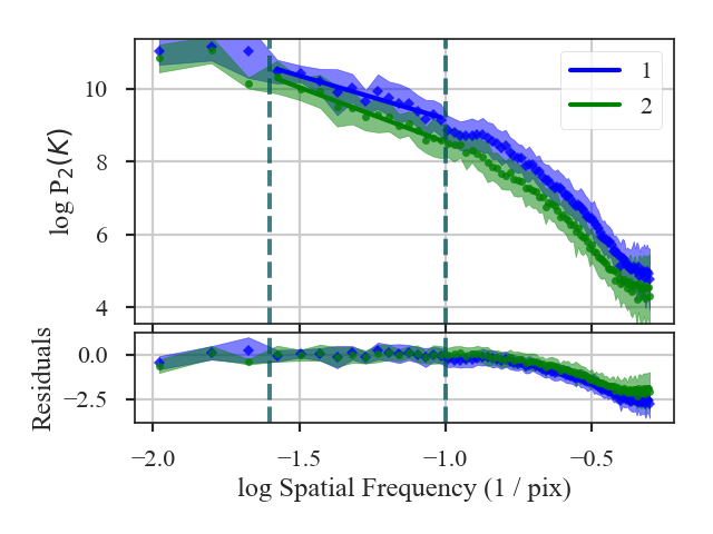
The fit summaries and a plot of the power-spectra with their fits are returned when verbose=True. Colours, labels, and symbols can be altered in the plot with the keywords plot_kwargs1 and plot_kwargs2 in distance_metric.
- The distance between these two images is:
>>> pspec.distance # doctest: +SKIP 3.0952798493530262
Recomputing an already compute power-spectrum can be avoided by passing a pre-computed PowerSpectrum instead of a dataset. See the distance metric introduction.
SCF Distance
See the tutorial for a description of the Spectral Correlation Function (SCF).
The SCF creates a surface by shifting a spectral-line cube and calculating the correlation of the shifted cube with the original cube. The distance metric defined in SCF_Distance is the L2 distance between the correlation surfaces, weighted by the inverse of the lag:
where \(S_i\) is the correlation surface and \(\ell\) is the spatial lag between the shifted and original cubes.
This direct comparison between the correlation surfaces requires that a common set of spatial lags be used. SCF_Distance creates a common set of angular lags to compare two data cubes.
More information on the distance metric definitions can be found in Koch et al. 2017
Using
The data in this tutorial are available here.
We need to import the SCF_Distance class, along with a few other common packages:
>>> from turbustat.statistics import SCF_Distance
>>> from astropy.io import fits
>>> import matplotlib.pyplot as plt
SCF_Distance takes two data cubes as input:
>>> cube = fits.open("Design4_flatrho_0021_00_radmc.fits")[0] # doctest: +SKIP
>>> cube_fid = fits.open("Fiducial0_flatrho_0021_00_radmc.fits")[0] # doctest: +SKIP
>>> scf = SCF_Distance(cube_fid, cube, size=11) # doctest: +SKIP
This call runs SCF for the two cubes, which can be accessed with scf1 and scf2.
The default setting assumes that the boundaries are continuous (e.g., simulated observations from a periodic-box simulation, like this example). To change how boundaries are handled, boundary can be set in SCF_Distance. For example, for observational data, boundary='cut' should be used. When comparing a simulated observation to a real observation, different boundary conditions can be given: boundary=['cut', 'continuous']. The first list item will be used for the first cube given to SCF_Distance and the same for the second list item.
To calculate the distance between the cubes:
>>> scf.distance_metric(verbose=True) # doctest: +SKIP
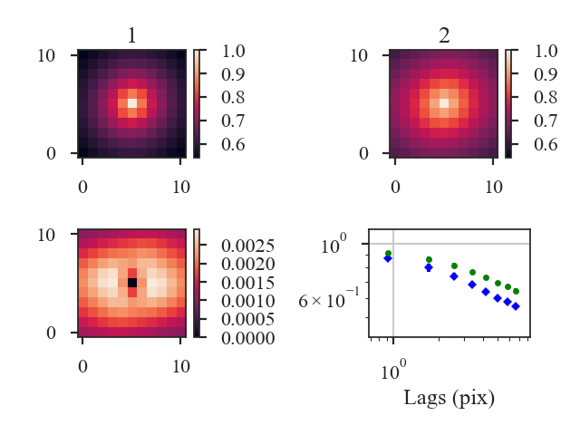
With verbose=True, this function creates a plot of the SCF correlation surfaces (top row), the weighted difference between the surfaces (left, second row), and azimuthally-averaged SCF curves for both cubes (right, second row).
The distance between the SCF surfaces is:
>>> scf.distance # doctest: +SKIP
0.08101015924738914
By default, the distance between the surfaces is weighted by the lag (see equation above). This weighting can be disabled by setting weighted=False in distance_metric, and the distance metrics reduces to the L2 norm between the surfaces.
A pre-computed SCF class can be also passed instead of a data cube. However, the SCF will need to be recomputed if the lags are different from the common set defined in SCF_Distance. See the distance metric introduction.
Statistical Moments Distance
See the tutorial for a description of the statistics moments.
StatsMoments calculates the first four moments—the mean, variance, skewness, and kurtosis—in circular regions of a map. For comparisons between different images, we utilize the skewness and kurtosis as metrics since they are not affected by offsets in the mean and are normalized by the variance. We reduce the moment images to histograms and define metrics from differences in the histograms. The histogram difference is converted to a distance by using the Hellinger distance:
where \(p_i\) is the histogram of an image and \(\tilde{I}\) is the bin of the histogram. The same definition is used for the skewness and kurtosis.
More information on the distance metric definitions can be found in Koch et al. 2017
Using
The data in this tutorial are available here.
We need to import the StatMoments_Distance class, along with a few other common packages:
>>> from turbustat.statistics import StatMoments_Distance
>>> from astropy.io import fits
>>> import matplotlib.pyplot as plt
>>> import astropy.units as u
And we load in the two data sets; in this case, two integrated intensity (zeroth moment) maps:
>>> moment0 = fits.open("Design4_flatrho_0021_00_radmc_moment0.fits")[0] # doctest: +SKIP
>>> moment0_fid = fits.open("Fiducial0_flatrho_0021_00_radmc_moment0.fits")[0] # doctest: +SKIP
These images are given as inputs to StatMoments_Distance:
>>> moments = StatMoments_Distance(moment0_fid, moment0, radius=5 * u.pix,
... periodic1=True, periodic2=True) # doctest: +SKIP
This runs StatMoments for both images, which can be accessed with moments1 and moments2.
Since the moments are calculated in circular regions, it is important that the a common circular region be used for both images. StatMoments_Distance scales the given radius to a common angular scale using the WCS information in the headers.
The boundary handling can also be changed by setting periodic1 and periodic2 for the first and second images, respectively. By default, periodic boundaries are used, as is appropriated for simulated observations from a periodic-box (like this example). For real observations, periodic boundaries will likely need to be disabled.
To calculate the distance between the images:
>>> moments.distance_metric(verbose=True) # doctest: +SKIP
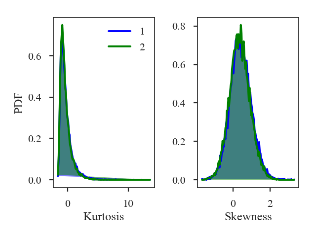
Additional arguments for the figure and the number of bins can also be given. The default number of bins for the histogram is set to \(\sqrt{{\rm min}(N_1, N_2)}\) where \(N_i\) is the number of pixels in each image with a finite value.
The distances for the skewness and kurtosis are:
>>> print(moments.skewness_distance, moments.kurtosis_distance) # doctest: +SKIP
0.01189910501201634 0.019870935761084074
A pre-computed StatMoments class can be passed instead of an image. However, the moments will need to be recomputed if the size differs from the common scale determined in StatMoments_Distance. See the distance metric introduction.
VCA Distance
See the tutorial for a description of Velocity Channel Analysis (VCA).
The VCA distance is defined as the t-statistic of the difference in the fitted slopes:
\(\beta_i\) are the slopes of the VCA spectra and \(\sigma_{\beta_i}\) are the uncertainty of the slopes.
More information on the distance metric definitions can be found in Koch et al. 2017.
Using
The data in this tutorial are available here.
We need to import the VCA_Distance class, along with a few other common packages:
>>> from turbustat.statistics import VCA_Distance
>>> from astropy.io import fits
>>> import matplotlib.pyplot as plt
>>> import astropy.units as u
VCA_Distance takes two data cubes as input:
>>> cube = fits.open("Design4_flatrho_0021_00_radmc.fits")[0] # doctest: +SKIP
>>> cube_fid = fits.open("Fiducial0_flatrho_0021_00_radmc.fits")[0] # doctest: +SKIP
From the VCA tutorial, we know that limits should be placed on the power-spectra. These limits can be specified with low_cut and high_cut:
>>> vca = VCA_Distance(cube_fid, cube, low_cut=0.025 / u.pix,
... high_cut=0.1 / u.pix) # doctest: +SKIP
This will run VCA on the given cubes, which can be accessed as vca1 and vca2.
Additional parameters can be specified to VCA. Different fit limits for the two cubes can be given as a two-element list (e.g., low_cut=[0.025 / u.pix, 0.04 / u.pix]). Estimated break points in the power-spectra can be given in the same format, which will enable fitting with a broken-linear model.
- To find the distance between the cubes:
>>> vca.distance_metric(verbose=True) # doctest: +SKIP OLS Regression Results ============================================================================== Dep. Variable: y R-squared: 0.985 Model: OLS Adj. R-squared: 0.984 Method: Least Squares F-statistic: 436.3 Date: Fri, 16 Nov 2018 Prob (F-statistic): 8.40e-11 Time: 10:16:28 Log-Likelihood: 22.506 No. Observations: 14 AIC: -41.01 Df Residuals: 12 BIC: -39.73 Df Model: 1 Covariance Type: HC3 ============================================================================== coef std err z P>|z| [0.025 0.975] ------------------------------------------------------------------------------ const 5.0853 0.137 37.170 0.000 4.817 5.353 x1 -2.3350 0.112 -20.887 0.000 -2.554 -2.116 ============================================================================== Omnibus: 0.981 Durbin-Watson: 1.483 Prob(Omnibus): 0.612 Jarque-Bera (JB): 0.712 Skew: -0.138 Prob(JB): 0.700 Kurtosis: 1.930 Cond. No. 15.2 ============================================================================== OLS Regression Results ============================================================================== Dep. Variable: y R-squared: 0.986 Model: OLS Adj. R-squared: 0.985 Method: Least Squares F-statistic: 722.3 Date: Fri, 16 Nov 2018 Prob (F-statistic): 4.33e-12 Time: 10:16:28 Log-Likelihood: 18.704 No. Observations: 14 AIC: -33.41 Df Residuals: 12 BIC: -32.13 Df Model: 1 Covariance Type: HC3 ============================================================================== coef std err z P>|z| [0.025 0.975] ------------------------------------------------------------------------------ const 3.6086 0.141 25.636 0.000 3.333 3.884 x1 -3.2136 0.120 -26.876 0.000 -3.448 -2.979 ============================================================================== Omnibus: 13.847 Durbin-Watson: 2.394 Prob(Omnibus): 0.001 Jarque-Bera (JB): 9.666 Skew: -1.631 Prob(JB): 0.00796 Kurtosis: 5.434 Cond. No. 15.2 ==============================================================================
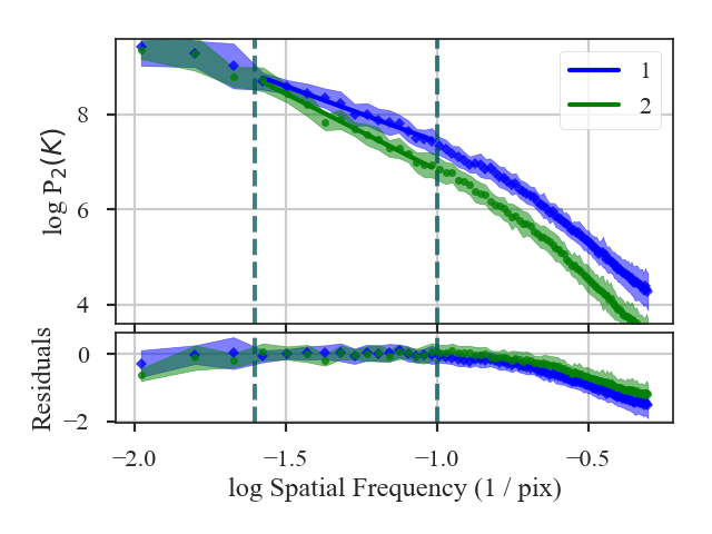
This function returns a summary of the fits to the VCA spectra and plots the two spectra with the fits. Colours, symbols and labels in the plot can be changed with plot_kwargs1 and plot_kwargs2 in distance_metric.
- The distance is:
>>> vca.distance # doctest: +SKIP 5.366955632554179
Changing the width of the velocity channels affects the contribution of the turbulent velocity field to the spectrum, thereby altering the measured index (Lazarian & Pogosyan 2000). It is generally advisable to compare cubes with a similar velocity resolution.
In VCA_Distance, the channel width can be changed with channel_width. The new channel width should be (1) larger than the current channel widths of the cubes, and (2) in similar units to the spectral axis of the cubes (i.e., a width in velocity should be given for a spectral axis in velocity).
Warning
Changing the spectral resolution will be slow for large cubes. Consider changing the velocity resolution of large cubes before running VCA.
In this example, we will change the velocity resolution to 400 m/s:
>>> vca = VCA_Distance(cube_fid, cube, low_cut=0.025 / u.pix,
... high_cut=0.1 / u.pix, channel_width=400 * u.m / u.s) # doctest: +SKIP
>>> vca.distance_metric(verbose=True) # doctest: +SKIP
OLS Regression Results
==============================================================================
Dep. Variable: y R-squared: 0.985
Model: OLS Adj. R-squared: 0.983
Method: Least Squares F-statistic: 419.3
Date: Fri, 16 Nov 2018 Prob (F-statistic): 1.06e-10
Time: 10:16:28 Log-Likelihood: 22.121
No. Observations: 14 AIC: -40.24
Df Residuals: 12 BIC: -38.96
Df Model: 1
Covariance Type: HC3
==============================================================================
coef std err z P>|z| [0.025 0.975]
------------------------------------------------------------------------------
const 3.0105 0.141 21.350 0.000 2.734 3.287
x1 -2.3639 0.115 -20.478 0.000 -2.590 -2.138
==============================================================================
Omnibus: 0.854 Durbin-Watson: 1.515
Prob(Omnibus): 0.652 Jarque-Bera (JB): 0.676
Skew: -0.144 Prob(JB): 0.713
Kurtosis: 1.963 Cond. No. 15.2
==============================================================================
OLS Regression Results
==============================================================================
Dep. Variable: y R-squared: 0.985
Model: OLS Adj. R-squared: 0.984
Method: Least Squares F-statistic: 684.5
Date: Fri, 16 Nov 2018 Prob (F-statistic): 5.94e-12
Time: 10:16:28 Log-Likelihood: 17.855
No. Observations: 14 AIC: -31.71
Df Residuals: 12 BIC: -30.43
Df Model: 1
Covariance Type: HC3
==============================================================================
coef std err z P>|z| [0.025 0.975]
------------------------------------------------------------------------------
const 1.5197 0.146 10.408 0.000 1.234 1.806
x1 -3.2379 0.124 -26.163 0.000 -3.481 -2.995
==============================================================================
Omnibus: 13.778 Durbin-Watson: 2.379
Prob(Omnibus): 0.001 Jarque-Bera (JB): 9.575
Skew: -1.633 Prob(JB): 0.00833
Kurtosis: 5.398 Cond. No. 15.2
==============================================================================
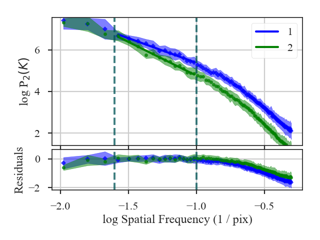
The VCA power-spectra with 400 m/s channels have a similar slope to the original velocity resolution. The distance then has not significantly changed:
>>> vca.distance # doctest: +SKIP
5.164776059129051
A pre-computed VCA class can be also passed instead of a data cube. See the distance metric introduction.
VCS Distance
See the tutorial for a description of Velocity Coordinate Spectrum (VCS).
There are two asymptotic regimes of the VCS corresponding to high and low resolution (Lazarian & Pogosyan 2006). The transition between these regimes depends on the spatial resolution (i.e., beam size) of the data, the spectral resolution of the data, and the velocity dispersion. The current VCS implementation in TurbuStat fits a broken linear model to approximate the asymptotic regimes, rather than fitting with the full VCS formalism (Chepurnov et al. 2010, Chepurnov et al. 2015). We assume that the break point lies at the transition point between the regimes and label velocity frequencies smaller than the break as “large-scale” and frequencies larger than the break as “small-scale”.
There are four distance definitions for the VCS based on the broken linear modelling described above. All of these distance metrics are based on t-statistics between the VCS for each cube:
- The difference between the fitted slopes on “large-scales” (below the break position):
large_scale_distance. - \[d_{\rm large-scale} = \frac{|\beta_{{\rm LS}, 1} - \beta_{{\rm LS}, 2}|}{\sqrt{\sigma_{\beta_{{\rm LS}, 1}}^2 + \sigma_{\beta_{{\rm LS}, 2}}^2}}\]
\(\beta_{{\rm LS}, i}\) are the slopes of the VCS on large-scales and \(\sigma_{\beta_{{\rm LS}, i}}\) are the uncertainty of the slopes.
- The difference between the fitted slopes on “large-scales” (below the break position):
- The difference between the fitted slopes on “small-scales” (above the break position):
small_scale_distance. - \[d_{\rm small-scale} = \frac{|\beta_{{\rm SS}, 1} - \beta_{{\rm SS}, 2}|}{\sqrt{\sigma_{\beta_{{\rm SS}, 1}}^2 + \sigma_{\beta_{{\rm SS}, 2}}^2}}\]
\(\beta_{{\rm SS}, i}\) are the slopes of the VCS on small-scales and \(\sigma_{\beta_{{\rm SS}, i}}\) are the uncertainty of the slopes.
- The difference between the fitted slopes on “small-scales” (above the break position):
- The sum of the differences between the slopes in both regimes:
distance - \[d_{{\rm all}} = d_{\rm large-scale} + d_{\rm small-scale}\]
- The sum of the differences between the slopes in both regimes:
- The difference in the fitted break points:
break_distance - \[d_{\rm break} = \frac{|b_{1} - b_{2}|}{\sqrt{\sigma_{b_{1}}^2 + \sigma_{b_{2}}^2}}\]
\(b_{i}\) are the break locations of the VCS and \(\sigma_{b_{i}}\) are the uncertainties.
- The difference in the fitted break points:
More information on the distance metric definitions can be found in Koch et al. 2017.
Using
The data in this tutorial are available here.
We need to import the VCS_Distance class, along with a few other common packages:
>>> from turbustat.statistics import VCS_Distance
>>> from astropy.io import fits
>>> import matplotlib.pyplot as plt
>>> import astropy.units as u
VCS_Distance takes two data cubes as input:
>>> cube = fits.open("Design4_flatrho_0021_00_radmc.fits")[0] # doctest: +SKIP
>>> cube_fid = fits.open("Fiducial0_flatrho_0021_00_radmc.fits")[0] # doctest: +SKIP
From the VCS tutorial, we know that limits should be placed on the power-spectra. These limits can be specified with low_cut and high_cut:
>>> vcs = VCS_Distance(cube_fid, cube,
... fit_kwargs=dict(low_cut=0.025 / u.pix,
... high_cut=0.1 / u.pix)) # doctest: +SKIP
This will run VCS on the given cubes, which can be accessed as vcs1 and vcs2.
Settings for the VCS fitting can be passed with fit_kwargs, and fit_kwargs2 when different setting are required for the second cube. In this example, we set the fitting limits to be used.
- To find the distances between the cube:
>>> vcs.distance_metric(verbose=True) # doctest: +SKIP OLS Regression Results ============================================================================== Dep. Variable: y R-squared: 0.993 Model: OLS Adj. R-squared: 0.992 Method: Least Squares F-statistic: 3678. Date: Fri, 16 Nov 2018 Prob (F-statistic): 1.96e-86 Time: 11:20:09 Log-Likelihood: -17.089 No. Observations: 85 AIC: 42.18 Df Residuals: 81 BIC: 51.95 Df Model: 3 Covariance Type: nonrobust ============================================================================== coef std err t P>|t| [0.025 0.975] ------------------------------------------------------------------------------ const 1.2848 0.295 4.354 0.000 0.698 1.872 x1 -2.1220 0.171 -12.428 0.000 -2.462 -1.782 x2 -14.5354 0.317 -45.812 0.000 -15.167 -13.904 x3 0.0715 0.129 0.553 0.582 -0.186 0.329 ============================================================================== Omnibus: 2.570 Durbin-Watson: 0.089 Prob(Omnibus): 0.277 Jarque-Bera (JB): 2.546 Skew: -0.378 Prob(JB): 0.280 Kurtosis: 2.616 Cond. No. 21.5 ============================================================================== OLS Regression Results ============================================================================== Dep. Variable: y R-squared: 0.988 Model: OLS Adj. R-squared: 0.987 Method: Least Squares F-statistic: 2212. Date: Fri, 16 Nov 2018 Prob (F-statistic): 1.43e-77 Time: 11:20:09 Log-Likelihood: -38.551 No. Observations: 85 AIC: 85.10 Df Residuals: 81 BIC: 94.87 Df Model: 3 Covariance Type: nonrobust ============================================================================== coef std err t P>|t| [0.025 0.975] ------------------------------------------------------------------------------ const 1.5246 0.380 4.014 0.000 0.769 2.280 x1 -1.9578 0.220 -8.908 0.000 -2.395 -1.520 x2 -14.7109 0.408 -36.020 0.000 -15.524 -13.898 x3 0.1178 0.167 0.707 0.482 -0.214 0.449 ============================================================================== Omnibus: 7.714 Durbin-Watson: 0.059 Prob(Omnibus): 0.021 Jarque-Bera (JB): 3.123 Skew: -0.127 Prob(JB): 0.210 Kurtosis: 2.096 Cond. No. 21.5 ==============================================================================
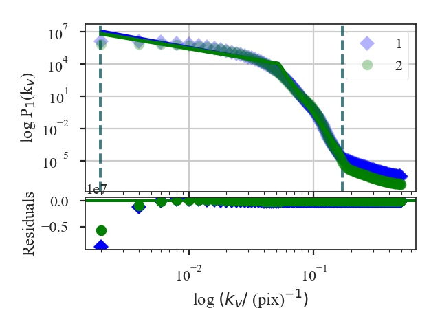
This function returns a summary of the broken linear fits to the VCS for each cube. The plot shows the VCS for both cubes; in this example, the two are quite similar.
The distances between the cubes, as defined above, are:
>>> vcs.large_scale_distance # doctest: +SKIP
0.5901343561262037
>>> vcs.small_scale_distance # doctest: +SKIP
0.01921401163828633
>>> vcs.distance # doctest: +SKIP
0.60934836776449
>>> vcs.break_distance # doctest: +SKIP
0.0023172070537929865
The difference in the slopes is dominated by vcs.large_scale_distance, while the small-scale slopes are quite similar. The break locations are also similar and give a small vcs.break_distance.
A pre-computed VCS class can be also passed instead of a data cube. See the distance metric introduction.
Wavelet Distance
See the tutorial for a description of Delta-Variance.
The distance metric for wavelets is Wavelet_Distance. The distance is defined as the t-statistic of the difference between the slopes of the wavelet transforms:
\(\beta_i\) are the slopes of the wavelet transforms and \(\sigma_{\beta_i}\) are the uncertainty of the slopes.
More information on the distance metric definitions can be found in Koch et al. 2017
Using
The data in this tutorial are available here.
We need to import the Wavelet_Distance class, along with a few other common packages:
>>> from turbustat.statistics import Wavelet
>>> from astropy.io import fits
>>> import matplotlib.pyplot as plt
>>> import astropy.units as u
And we load in the two data sets; in this case, two integrated intensity (zeroth moment) maps:
>>> moment0 = fits.open("Design4_flatrho_0021_00_radmc_moment0.fits")[0] # doctest: +SKIP
>>> moment0_fid = fits.open("Fiducial0_flatrho_0021_00_radmc_moment0.fits")[0] # doctest: +SKIP
The two images are input to Wavelet_Distance:
>>> wavelet = Wavelet_Distance(moment0_fid, moment0, xlow=2 * u.pix,
... xhigh=10 * u.pix) # doctest: +SKIP
This call will run Wavelet on both of the images, which can be accessed with wt1 and wt2.
In this example, we have limited the fitting regions with xlow and xhigh. Separate fitting limits for each image can be given by giving a two-element list for either keywords (e.g., xlow=[1 * u.pix, 2 * u.pix]). Additional fitting keyword arguments can be passed with fit_kwargs and fit_kwargs2 for the first and second images, respectively.
To calculate the distance:
>>> delvar.distance_metric(verbose=True, xunit=u.pix) # doctest: +SKIP
OLS Regression Results
==============================================================================
Dep. Variable: y R-squared: 0.983
Model: OLS Adj. R-squared: 0.982
Method: Least Squares F-statistic: 1013.
Date: Fri, 16 Nov 2018 Prob (F-statistic): 1.31e-18
Time: 17:55:59 Log-Likelihood: 73.769
No. Observations: 22 AIC: -143.5
Df Residuals: 20 BIC: -141.4
Df Model: 1
Covariance Type: HC3
==============================================================================
coef std err z P>|z| [0.025 0.975]
------------------------------------------------------------------------------
const 1.5636 0.006 267.390 0.000 1.552 1.575
x1 0.3137 0.010 31.832 0.000 0.294 0.333
==============================================================================
Omnibus: 3.421 Durbin-Watson: 0.195
Prob(Omnibus): 0.181 Jarque-Bera (JB): 1.761
Skew: -0.397 Prob(JB): 0.414
Kurtosis: 1.864 Cond. No. 7.05
==============================================================================
OLS Regression Results
==============================================================================
Dep. Variable: y R-squared: 0.993
Model: OLS Adj. R-squared: 0.993
Method: Least Squares F-statistic: 1351.
Date: Fri, 16 Nov 2018 Prob (F-statistic): 7.76e-20
Time: 17:55:59 Log-Likelihood: 75.406
No. Observations: 22 AIC: -146.8
Df Residuals: 20 BIC: -144.6
Df Model: 1
Covariance Type: HC3
==============================================================================
coef std err z P>|z| [0.025 0.975]
------------------------------------------------------------------------------
const 1.3444 0.008 158.895 0.000 1.328 1.361
x1 0.4728 0.013 36.752 0.000 0.448 0.498
==============================================================================
Omnibus: 4.214 Durbin-Watson: 0.170
Prob(Omnibus): 0.122 Jarque-Bera (JB): 3.493
Skew: -0.958 Prob(JB): 0.174
Kurtosis: 2.626 Cond. No. 7.05
==============================================================================
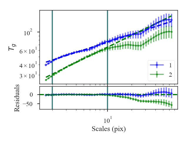
A summary of the fits are printed along with a plot of the two wavelet transforms and the fit residuals. Colours, labels, and symbols can be specified in the plot with plot_kwargs1 and plot_kwargs2.
The distances between these two datasets are:
>>> wavelet.curve_distance # doctest: +SKIP
9.81949754947785
A pre-computed Wavelet class can be also passed instead of a data cube. See the distance metric introduction.
Creating testing data
TurbuStat includes a simulation package to create 2D images and PPV cubes with set power-law indices. These provide simple non-realistic synthetic observations that can be used to test idealized regimes of turbulent statistics.:
>>> import matplotlib.pyplot as plt
>>> from astropy.io import fits
Two-dimensional images
- The 2D power-law image function is
make_extended:: >>> from turbustat.simulator import make_extended
The make_extended function is adapted from the implementation in image_registration.
To create an isotropic power-law field, or a fractional Brownian Motion (fBM) field, with an index of 3 and size of 256 pixels, we run:
>>> rnoise_img = make_extended(256, powerlaw=3.)
>>> plt.imshow(rnoise_img) # doctest: +SKIP
To calculate the power-spectrum and check its index, we need to generate a minimal FITS HDU:
>>> rnoise_hdu = fits.PrimaryHDU(rnoise_img)
The FITS header lacks the information to convert to angular or physical scales and is used here to show the minimal working case. See the handling simulated data tutorial on how to create usable FITS header for simulated data.
The power-spectrum of the image should give a slope of 3:
>>> from turbustat.statistics import PowerSpectrum
>>> pspec = PowerSpectrum(rnoise_hdu)
>>> pspec.run(verbose=True, radial_pspec_kwargs={'binsize': 1.0},
... fit_kwargs={'weighted_fit': True}, fit_2D=False,
... low_cut=1. / (60 * u.pix)) # doctest: +SKIP
OLS Regression Results
==============================================================================
Dep. Variable: y R-squared: 1.000
Model: OLS Adj. R-squared: 1.000
Method: Least Squares F-statistic: 8.070e+06
Date: Thu, 21 Jun 2018 Prob (F-statistic): 0.00
Time: 11:43:47 Log-Likelihood: 701.40
No. Observations: 177 AIC: -1399.
Df Residuals: 175 BIC: -1392.
Df Model: 1
Covariance Type: nonrobust
==============================================================================
coef std err t P>|t| [0.025 0.975]
------------------------------------------------------------------------------
const 0.0032 0.001 3.952 0.000 0.002 0.005
x1 -2.9946 0.001 -2840.850 0.000 -2.997 -2.992
==============================================================================
Omnibus: 252.943 Durbin-Watson: 1.077
Prob(Omnibus): 0.000 Jarque-Bera (JB): 26797.433
Skew: -5.963 Prob(JB): 0.00
Kurtosis: 62.087 Cond. No. 4.55
==============================================================================
Anisotropic 2D images can also be produced:
>>> import astropy.units as u
>>> rnoise_img = make_extended(256, powerlaw=3., ellip=0.5, theta=45 * u.deg)
>>> plt.imshow(rnoise_img) # doctest: +SKIP
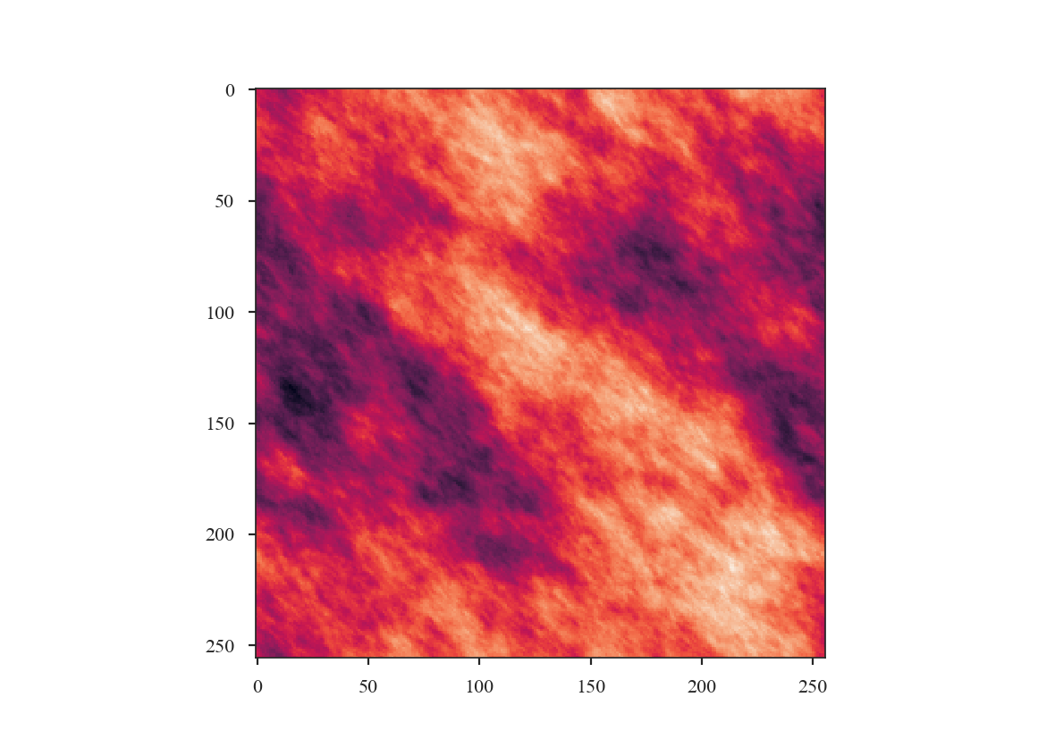
The power-spectrum can then be calculated and fit in 1D and 2D (see Spatial Power Spectrum):
>>> pspec = PowerSpectrum(rnoise_hdu)
>>> pspec.run(verbose=True, radial_pspec_kwargs={'binsize': 1.0},
... fit_kwargs={'weighted_fit': True}, fit_2D=False,
... low_cut=1. / (60 * u.pix)) # doctest: +SKIP
OLS Regression Results
==============================================================================
Dep. Variable: y R-squared: 1.000
Model: OLS Adj. R-squared: 1.000
Method: Least Squares F-statistic: 1.122e+06
Date: Wed, 15 Aug 2018 Prob (F-statistic): 0.00
Time: 14:18:14 Log-Likelihood: 526.68
No. Observations: 177 AIC: -1049.
Df Residuals: 175 BIC: -1043.
Df Model: 1
Covariance Type: nonrobust
==============================================================================
coef std err t P>|t| [0.025 0.975]
------------------------------------------------------------------------------
const 2.7786 0.002 1295.906 0.000 2.774 2.783
x1 -2.9958 0.003 -1059.077 0.000 -3.001 -2.990
==============================================================================
Omnibus: 35.156 Durbin-Watson: 2.661
Prob(Omnibus): 0.000 Jarque-Bera (JB): 334.753
Skew: 0.205 Prob(JB): 2.04e-73
Kurtosis: 9.725 Cond. No. 4.55
==============================================================================
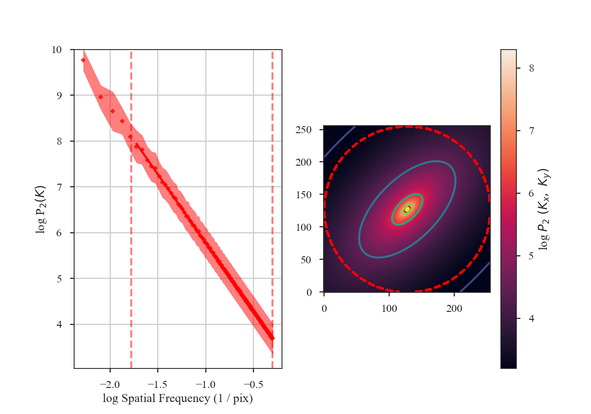
Three-dimensional fields
Three-dimensional power-law fields can also be produced with make_3dfield:
>>> from turbustat.simulator import make_3dfield
>>> threeD_field = make_3dfield(128, powerlaw=3.)
Only isotropic fields can currently be created. Projections of this 3D field are shown below:
>>> plt.figure(figsize=[10, 3]) # doctest: +SKIP
>>> plt.subplot(131) # doctest: +SKIP
>>> plt.imshow(threeD_field.mean(0), origin='lower') # doctest: +SKIP
>>> plt.subplot(132) # doctest: +SKIP
>>> plt.imshow(threeD_field.mean(1), origin='lower') # doctest: +SKIP
>>> plt.subplot(133) # doctest: +SKIP
>>> plt.imshow(threeD_field.mean(2), origin='lower') # doctest: +SKIP
>>> plt.tight_layout() # doctest: +SKIP
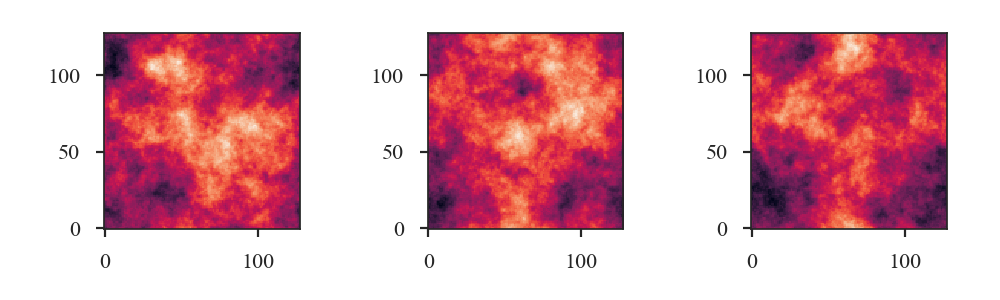
Simple PPV cubes
Also included in this module is a simple PPV cube generator. It has many restrictions and is primarily intended for creating idealized optically-thin 21-cm HI emission to test turbulent statistics in idealized conditions.
The function to create the cubes is:
>>> from turbustat.simulator import make_3dfield, make_ppv
>>> import astropy.units as u
We need to create 3D velocity and density cubes. For this simple example, we will create small 32 pixel cubes so this is quick to compute:
>>> velocity = make_3dfield(32, powerlaw=4., amp=1.,
... randomseed=98734) * u.km / u.s # doctest: +SKIP
>>> density = make_3dfield(32, powerlaw=3., amp=1.,
... randomseed=328764) * u.cm**-3 # doctest: +SKIP
Both fields need to have appropriate units.
There is an additional issue for the density field generated from a power-law in that it will contain negative values. There are numerous approaches to account for negative values, including adding the minimum to force all values to be positive or taking the exponential of this field to produce a log-normal field (Brunt & Heyer 2002, Roman-Duval et al. 2011). Here we use the approach from Ossenkopf et al. 2006, adding one standard deviation to all values and masking values that remain negative. Each of these approaches will distort the field properties to some extent.
>>> density += density.std() # doctest: +SKIP
>>> density[density.value < 0.] = 0. * u.cm**-3 # doctest: +SKIP
To produce a PPV cube from these fields, using the zeroth axis as the line-of-sight:
>>> cube_hdu = make_ppv(velocity, density, los_axis=0,
... T=100 * u.K, chan_width=0.5 * u.km / u.s,
... v_min=-20 * u.km / u.s,
... v_max=20 * u.km / u.s) # doctest: +SKIP
We will demonstrate the cube properties using spectral-cube:
>>> from spectral_cube import SpectralCube # doctest: +SKIP
>>> cube = SpectralCube.read(cube_hdu) # doctest: +SKIP
The zeroth moment, integrated over the velocity axis:
>>> cube.moment0().quicklook() # doctest: +SKIP
>>> plt.colorbar() # doctest: +SKIP
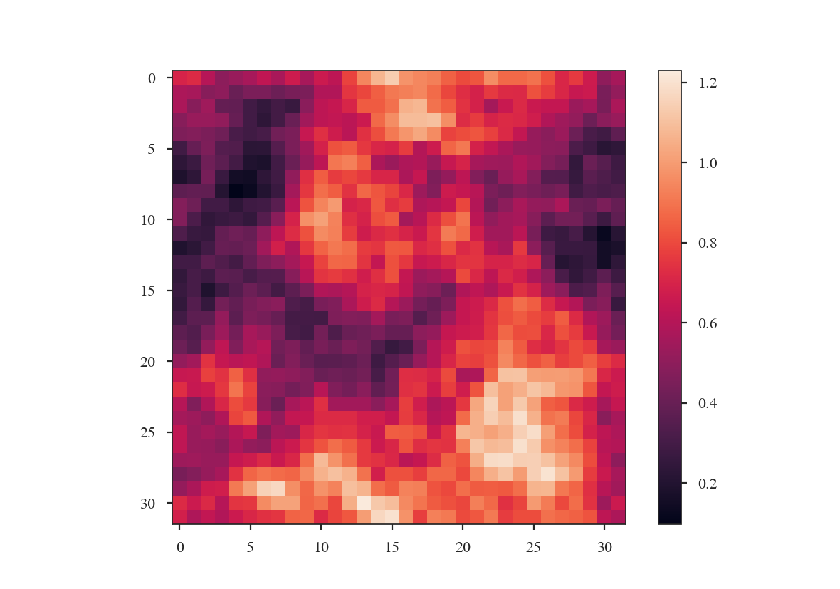
The velocity centroid map:
>>> cube.moment1().quicklook() # doctest: +SKIP
>>> plt.colorbar() # doctest: +SKIP
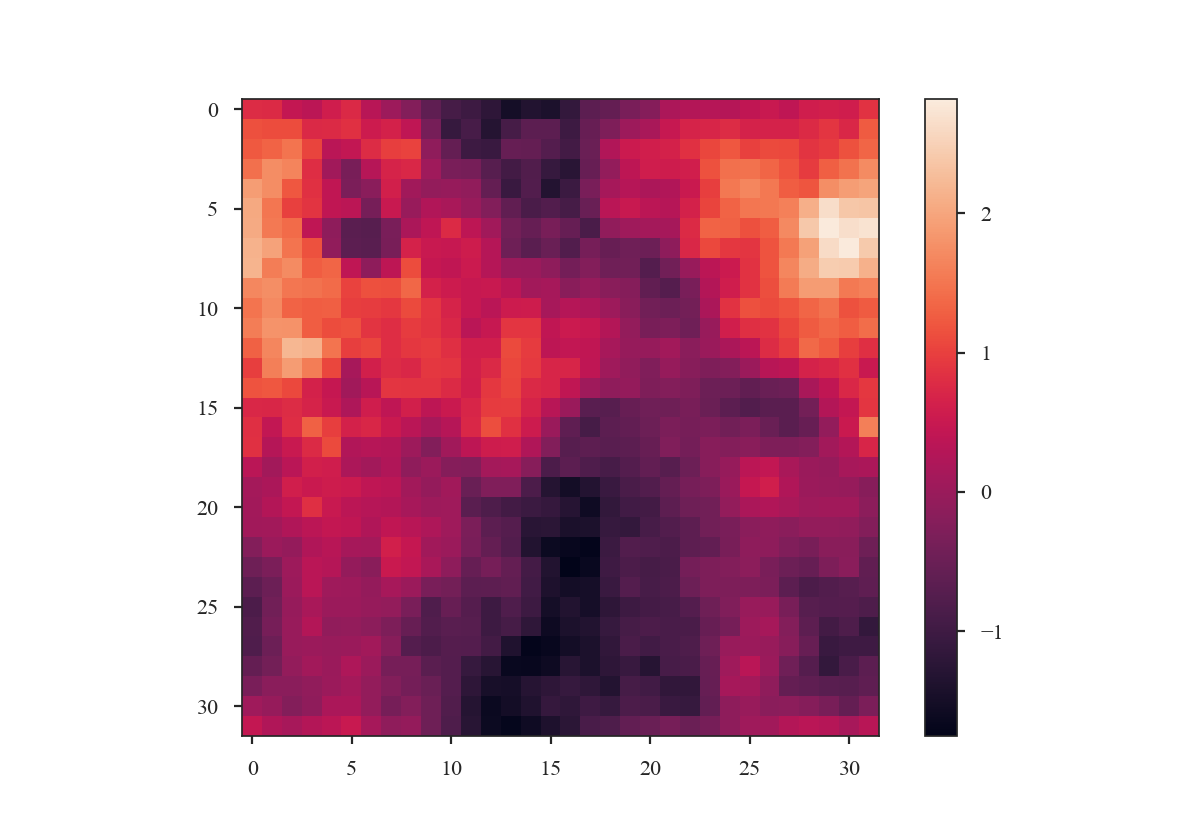
And the mean spectrum, averaged over the spatial dimensions:
>>> cube.mean(axis=(1, 2)).quicklook() # doctest: +SKIP
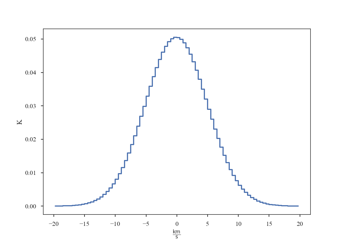
Warning
These simulated cubes (and those from other numerical methods) will suffer from “shot noise” due to a finite number of emitting sources along the line of sight. This will lead to deviations of expected behaviours for several statistics, most notably the VCA and VCS methods. See Esquivel et al. 2003 and Chepurnov et al. 2009 for thorough explanations of this effect.
Useful references for making mock-HI cubes include:
Source Code
Functions
make_3dfield(imsize[, powerlaw, amp, …]) |
Generate a 3D power-law field with a specified index and random phases. |
make_extended(imsize[, powerlaw, theta, …]) |
Generate a 2D power-law image with a specified index and random phases. |
make_ppv(vel_field, dens_field[, los_axis, …]) |
Generate a mock, optically-thin HI PPV cube from a given velocity and density field. |
Statistics
Along with acting as the base classes for the distance metrics, the statistics can also return useful information about single datasets. See the Using statistics classes tutorial for more information on computing Statistics.
Distance Metrics
The distance metrics are computed using certain outputs contained in the related statistics class. See the Using distance metrics tutorial for more information on how to use Distance Metrics.
Nearly all of the distance metrics are actually “pseudo” - distance metrics. They must have the following properties:
- \(d(A, A) = 0\)
- Symmetric \(d(A, B) = d(B, A)\)
- Triangle Inequality \(d(A, B) \leq d(A, C) + d(B, C)\)
Here \(A\) and \(B\) represent two datasets (either a PPV datacube, column density map, or an associated moment of the cube).
For two datasets with different physical properties, a good statistic will return a large value \(d(A, B) \gg 0\). If the datasets have similar physical properties, the distance should be small \(d(A, B) \approx 0\). Clear examples of the distance metric properties and the distinction between large and small distances are shown in Boyden et al. 2016 and Boyden et al. 2018.
Additionally, the statistics should ideally be insensitive to spatial shifts \(d\left( A\left[ x,y,v \right], A\left[ x+\delta x,y,v \right] \right)=0\) and independent of the noise level (for observational data) \(d\left( A + \mathcal{N}\left(0, \sigma_1^2 \right), A + \mathcal{N}\left(0, \sigma_2^2 \right) \right) \approx 0\).
Source Code
turbustat.statistics Package
Functions
BiSpectrum(*args, **kwargs) |
Old name for the Bispectrum class. |
BiSpectrum_Distance(*args, **kwargs) |
Old name for the Bispectrum class. |
DendroDistance(*args, **kwargs) |
Old name for the Dendrogram_Distance class. |
GenusDistance(*args, **kwargs) |
Old name for the Genus_Distance class. |
WidthEstimate1D(inList[, method]) |
Find widths from spectral eigenvectors. |
WidthEstimate2D(inList[, method, noise_ACF, …]) |
Estimate spatial widths from a set of autocorrelation images. |
Classes
Bispectrum(img) |
Computes the bispectrum (three-point correlation function) of the given image (Burkhart et al., 2010). |
Bispectrum_Distance(data1, data2[, stat_kwargs]) |
Calculate the distance between two images based on their bicoherence. |
Cramer_Distance(cube1, cube2[, …]) |
Compute the Cramer distance between two data cubes. |
DeltaVariance(img[, header, weights, …]) |
The delta-variance technique as described in Ossenkopf et al. |
DeltaVariance_Distance(dataset1, dataset2[, …]) |
Compares 2 datasets using delta-variance. |
Dendrogram_Distance(dataset1, dataset2[, …]) |
Calculate the distance between 2 cubes using dendrograms. |
Dendrogram_Stats(data[, header, min_deltas, …]) |
Dendrogram statistics as described in Burkhart et al. |
Genus(img[, min_value, max_value, …]) |
Genus Statistics based off of Chepurnov et al. |
Genus_Distance(img1, img2[, …]) |
Distance Metric for the Genus Statistic. |
Lm_Seg(x, y, brk[, weights]) |
|
MVC(centroid, moment0, linewidth[, header, …]) |
Implementation of Modified Velocity Centroids (Lazarian & Esquivel, 03) |
MVC_Distance(data1, data2[, …]) |
Distance metric for MVC. |
PCA(cube[, n_eigs, distance]) |
Implementation of Principal Component Analysis (Heyer & Brunt, 2002) |
PCA_Distance(cube1, cube2[, n_eigs, …]) |
Compare two data cubes based on the eigenvalues of the PCA decomposition. |
PDF(img[, min_val, bins, weights, …]) |
Create the PDF of a given array. |
PDF_Distance(img1, img2[, min_val1, …]) |
Calculate the distance between two arrays using their PDFs. |
PSpec_Distance(data1, data2[, weights1, …]) |
Distance metric for the spatial power spectrum. |
PowerSpectrum(img[, header, weights, …]) |
Compute the power spectrum of a given image. |
SCF(cube[, header, size, roll_lags, distance]) |
Computes the Spectral Correlation Function of a data cube (Rosolowsky et al, 1999). |
SCF_Distance(cube1, cube2[, size, boundary, …]) |
Calculates the distance between two data cubes based on their SCF surfaces. |
StatMoments(img[, header, weights, radius, …]) |
Statistical Moments of an image. |
StatMoments_Distance(image1, image2[, …]) |
Compute the distance between two images based on their moments. |
Tsallis(img[, header, lags, distance]) |
The Tsallis Distribution (see Tofflemire et al., 2011) |
VCA(cube[, header, distance, beam, …]) |
The VCA technique (Lazarian & Pogosyan, 2004). |
VCA_Distance(cube1, cube2[, channel_width, …]) |
Calculate the distance between two cubes using VCA. |
VCS(cube[, header]) |
The VCS technique (Lazarian & Pogosyan, 2004). |
VCS_Distance(cube1, cube2[, breaks, …]) |
Calculate the distance between two cubes using VCS. |
Wavelet(data[, header, scales, num, distance]) |
Compute the wavelet transform of a 2D array. |
Wavelet_Distance(dataset1, dataset2[, …]) |
Compute the distance between the two cubes using the Wavelet transform. |
Contributing to TurbuStat
We welcome new contributions to TurbuStat!
To make changes to the source code, make a fork of the TurbuStat repository by pressing the button on the top right-hand side of the page. Changes to the code should be made in a new branch, pushed to your fork of the repository, and submitted with a pull request to the main TurbuStat repository. For more information and a detailed guide to using git, please see the astropy workflow page.
Contributing a new statistic or distance metric
Increasing the number of statistics implemented in TurbuStat is a key goal for the project. If you plan on providing a new implementation, the contribution should address the following criteria:
- Statistics and distance metrics should be a python class. A new folder can be added to the statistics folder for the new classes. Note that the new folder should contain an
__init__.pythe imports the statistic and/or distance metric classes (see here for an example). - Statistics should inherit from the BaseStatisticMixIn class. This mixin class handles unit conversions, extracts the required information from the FITS header, and allows the class to be saved and loaded.
- Statistic classes should accept the required data products in
__init__. At a minimum, the class should require the data and a FITS header. Other parameters that define the data or observed object (e.g., distance) can also be specified here. Functions within the class should take the data and compute the statistic. For example, the spectral correlation function (SCF) has separate function to create the SCF surface, to make an azimuthally-averaged spectrum, to fit two-dimensional and one-dimensional, and to make a summary plot. - All statistic classes should have a
runfunction that computes the statistic and optionally returns a summary plot (e.g., for the SCF). Therunfunction should use sensible defaults, but should have keyword arguments defined for the most important parameters. - Distance classes should accept the required data for two data sets in
__init__. The statistic class should be run on both data sets and keyword arguments should allow the important parameters to be passed to the statistic class (e.g., for the SCF distance). The distance class should then have adistance_metricfunction defined (for example) that computes the distance metric and optionally returns a summary plot of the statistic run on both of the data sets. - New statistics and distance metrics should have documentation explaining each argument, keyword argument, parameter, and function in the class. TurbuStat follows the astropy docstring rules.
- New statistics and distance metrics must have consistency tests. There are two types of consistency tests in TurbuStat: (i) Unit tests against the small test data included in the package (see here). An output from the statistic and distance metric is saved when the GetVals.py script is run. This type of test determines whether new additions to the code/updates the dependent package change the statistic’s output. (ii) Simple model tests where the statistic’s output is known. For example, the power-spectrum can be tested by generating an fBM image with a specified index (e.g., see this test).
- New statistics and distance metrics should have a tutorial for users (e.g., see this tutorial). Ideally, the tutorial will use the data sets already used in the TurbuStat tutorials. If these data are not useful for demonstrating the new statistic, we ask that the tutorial data be (i) small so the computation is relatively quick to run and (ii) publicly-available so users can reproduce the tutorial results.